Level I Equity

Access to all Level I equity articles until the next Level I exam date

A time-honored method to determine the value of an investment is to discount to the present all of the investment’s (expected) future cash flows, and tot up those present values.  It’s a method we use commonly when valuing bonds, and when valuing projects in which a company is considering investing (e.g., whether or not to purchase a machine that makes tennis balls): calculating the net present value (NPV), or, in a similar vein, its internal rate of return (IRR).  I describe these ideas in detail in this article.

Extending that idea to an investment in a company’s stock, when a company pays dividends regularly – and is expected to continue to pay dividends ad infinitum – a reasonable way to determine the value of the company’s stock is to use a dividend discount model (DDM): discount each of the expected dividends to the present (at your required rate of return) and tot up those present values; the resulting sum is the value of the stock (at least, its value to you).

Example

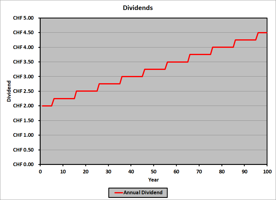
Euler Pharmaceuticals pays an annual dividend of CHF 2.00 per share.  Historically, they have raised their annual dividend by CHF 0.25 per share every 10 years; they have been paying the current dividend for the last 5 years.  Their expected dividends are:

Year Dividend
1 CHF 2.00
2 CHF 2.00
3 CHF 2.00
4 CHF 2.00
5 CHF 2.00
6 CHF 2.25
7 CHF 2.25
8 CHF 2.25
9 CHF 2.25
10 CHF 2.25
11 CHF 2.25
12 CHF 2.25
13 CHF 2.25
14 CHF 2.25
15 CHF 2.25

.

.

.

.

.

.

96 CHF 4.50
97 CHF 4.50
98 CHF 4.50
99 CHF 4.50
100 CHF 4.50

Graphically:

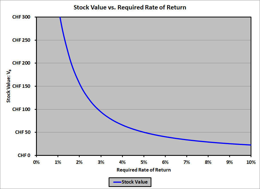
The value of the stock depends on the discount rate (required rate of return) used to determine the present value of the dividends.  The value versus the required rate of return is:

Required Return V0
0.0% $935.00
0.5% $529.11
1.0% $325.78
1.5% $217.43
2.0% $155.78
2.5% $118.33
3.0% $94.14
3.5% $77.61
4.0% $65.77
4.5% $56.94
5.0% $50.14
5.5% $44.75
6.0% $40.38
6.5% $36.78
7.0% $33.75
7.5% $31.18
8.0% $28.96
8.5% $27.04
9.0% $25.35
9.5% $23.86
10.0% $22.53

Graphically:

The problem with this (sort of) real-world example is that analyzing a dividend that increases every once in a while and otherwise remains constant is . . . um . . . difficult (unless you’re doing it in Excel, as I am).

Therefore, the curriculum makes some simplifying assumptions to make it easier to determine the value of a stock based on its expected dividends.  We acknowledge that these assumptions are unreasonable in the real world, but they make the models easy to understand.  Once you understand these simplified models thoroughly, it’s much easier to graduate to more complex (i.e., realistic) models and understand them.  So . . . tally ho!

(Short) Holding Period Models

We start with the most unrealistic model possible: you plan to buy a stock today, hold it for one year (receiving one dividend at the end of the year), then sell it.  You know your required rate of return, you know the dividend you’ll receive in one year, and you know the price at which you’ll be able to sell the stock in one year.  (That’s the unreasonable part: how can you possibly know the price at which you’ll sell the stock in one year without knowing its price today?)  You need to compute the price of the stock today.  Let’s look again at Euler Pharmaceuticals:

  • Next year’s expected dividend: CHF 2.00
  • Expected price in one year: CHF 31.52
  • Required rate of return: 7.50%

The price you’d be willing to pay today is:

\begin{align}V_0\ &=\ \dfrac{D_1}{1 + r} + \dfrac{P_1}{1 + r}\\
\\
&=\ \dfrac{CHF\ 2.00}{1.075} + \dfrac{CHF\ 31.52}{1.075}\\
\\
&=\ CHF\ 1.86 + CHF\ 29.32\\
\\
&= CHF\ 31.18
\end{align}

Suppose, instead, that you plan to hold the stock for two years:

  • Expected dividend in one year: CHF 2.00
  • Expected dividend in two years: CHF 2.00
  • Expected price in two years: CHF 31.88
  • Required rate of return: 7.50%

The price you’d be willing to pay today is:

\begin{align}V_0\ &=\ \dfrac{D_1}{1 + r} + \dfrac{D_2}{\left(1 + r\right)^2} + \dfrac{P_2}{\left(1 + r\right)^2}\\
\\
&=\ \dfrac{CHF\ 2.00}{1.075} + \dfrac{CHF\ 2.00}{1.075^2} + \dfrac{CHF\ 31.88}{1.075^2}\\
\\
&=\ CHF\ 1.86 + CHF\ 1.73 + CHF\ 27.59\\
\\
&= CHF\ 31.18
\end{align}

Note that on your calculator, you can solve these with the TVM buttons.  For example, the second one can be solved this way: (with your calculator in END mode):

n = 2
i = 7.5%
PMT = 2.00
FV = 31.88
Solve for PV = −31.18

Single-Stage (Gordon Growth) Model

When the holding period is long-term (essentially, infinite, or perpetual), a common simplifying assumption is that the dividend grows at a constant rate.  The model incorporating this assumption is known as the Gordon Growth model, and the formula for the value of the stock is simplicity itself:

\begin{align}V_0\ &=\ \dfrac{D_1}{1 + r} + \dfrac{D_2}{\left(1 + r\right)^2} + \dfrac{D_3}{\left(1 + r\right)^3} + \cdots\\
\\
&= \sum_{i=1}^\infty \dfrac{D_i}{\left(1 + r\right)^i}\\
\\
&=\ \dfrac{D_0\left(1 + g\right)}{1 + r} + \dfrac{D_0\left(1 + g\right)^2}{\left(1 + r\right)^2} + \dfrac{D_0\left(1 + g\right)^3}{\left(1 + r\right)^3} + \cdots\\
\\
&= \sum_{i=1}^\infty \dfrac{D_0\left(1 + g\right)^i}{\left(1 + r\right)^i}\\
\\
V_0 &=\ \dfrac{D_0\left(1 + g\right)}{r\ -\ g} =\ \dfrac{D_1}{r\ -\ g}
\end{align}

where:

  • \(r\): required rate of return
  • \(g\): dividend growth rate

Note that this model makes sense only if \(r > g\).  Otherwise, the sum is infinite.

Let’s take a careful look at this formula, to see whether or not it makes sense.  We’ll compare the stocks of two companies, not particularly cleverly known as Company A and Company B.

D1

Suppose first that the stocks of Companies A and B are considered equally risky (so that they command the same required rate of return), and that their dividends will grow at the same rate unto perpetuity.  Company A just paid a dividend of GBP 1.00 while Company B just paid a dividend of GBP 1.25.  I hope that it’s clear that you would be willing to pay more for Company B’s stock than for Company A’s stock, and that’s exactly what we get from the Gordon Growth formula: when D0 (and, consequently, D1) is higher, all else equal, V0 is higher (because the numerator is bigger and the denominator is unchanged), and conversely.

r

Suppose now that Companies A and B just paid the same dividend, and that their dividends will grow at the same rate unto perpetuity, but that Company B’s stock is considered riskier than Company A’s stock.  I trust that it’s clear that your required rate of return for Company B’s stock will be higher than your required rate of return for Company A’s stock, and that, therefore, you would be willing to pay less for Company B’s stock than for Company A’s stock.  We see that that’s exactly what we get from the Gordon Growth formula: when r is higher, all else equal, V0 is lower (because the numerator is unchanged while the denominator is bigger), and conversely.

g

Suppose now that Companies A and B just paid the same dividend, and are considered equally risky, but that Company B’s dividend is expected to increase at a faster rate than Company A’s dividend.  I assume that it’s clear that you would be willing to pay more for Company B’s stock than for Company A’s stock.  We see that that’s exactly what we get from the Gordon Growth formula: when g is higher, all else equal, V0 is higher (because the numerator is unchanged while the denominator is smaller), and conversely.

In all cases, the Gordon Growth model passes muster: it behaves exactly as we should expect it to behave, and the analyses are simple and straightforward.  That’s the point of making these simplifying assumptions: it’s easy to understand how the model works, and it works the way it’s meant to work.  Once we understand that, presumably we can move on to more complex (and reasonable) models and be able to understand how they work as well.

Example

Suppose that Ramanujan Technologies just paid an annual dividend of INR 200.00 per share.  Its dividends are expected to grow at 1.5% per year, and you determine that 8.4% is an appropriate rate of return for such an investment.  The amount per share you should be willing to pay for Ramanujan Technologies stock is:

\[V_0 = \dfrac{D_1}{r\ -\ g} = \dfrac{INR\ 200 \times 1.015}{0.084\ -\ 0.015} = INR\ 2,942.03\]

Delayed Gordon Growth Model

Suppose that instead of the first dividend coming one year from today, we expect the first dividend five years from today; i.e., the company does not pay a dividend yet, but we expect that it will start paying one in five years (and that the dividend will grow at a constant rate thereafter).  Before we analyze the value of the company’s stock, let’s take another look at the Gordon Growth model:

\[V_0 = \dfrac{D_1}{r\ -\ g}\]

There’s nothing special about the subscript “0” on the value, or the subscript “1” on the dividend; what’s important is that the dividend comes one year after the date for the value.  So, for example,

\[V_1 = \dfrac{D_2}{r\ -\ g}\]

\[V_2 = \dfrac{D_3}{r\ -\ g}\]

and, in general,

\[V_t = \dfrac{D_{t+1}}{r\ -\ g}\]

Therefore, we can use the Gordon Growth model to determine the value of the stock one year before the first dividend is paid.  If the date on the value isn’t today, then we simply discount that value back to today.

Example

Suppose that Abel Industrial is expected to start paying a dividend five years from today.  The first (annual) dividend is anticipated to be EUR 2.50 per share, increasing 1% per year thereafter.  If your required rate of is 8.2%, how much would you be willing to pay for a share of Abel stock?

\begin{align}V_4\ &=\ \dfrac{D_5}{r\ -\ g}\\
\\
&= \dfrac{EUR\ 2.50}{8.2\%\ -\ 1.0\%}\\
\\
V_4 &= EUR\ 34.72\\
\\
V_0 &= \dfrac{V_4}{\left(1 + r\right)^4}\\
\\
&= \dfrac{EUR\ 34.72}{1.082^4}\\
\\
&=\ EUR\ 25.33
\end{align}

Multi-Stage Models

In a two-stage growth model, a company’s dividends are assumed to grow a one rate (presumably a high rate) for a finite period of time, then to grow at another rate (presumably a lower rate) forever thereafter.  In a three-stage growth model, the dividends are assumed to grow at one (high) rate for a finite period of time, then at a second (middling) rate for another finite period of time, then at a third (low) rate forever thereafter.  I’ll leave it to your imagination what a four-stage, or a five-stage, or a six-stage, or a more-than-six-stage model might be.

The approach for determining the value of the company’s stock under all of these models is the same:

  • Determine all of the dividend amounts for all of the finite periods
  • Discount those amounts to the present
  • Use the Delayed Gordon Growth model for the final (infinite) period
  • Tot up all of the present values
  • Voilà!

Two-Stage Example

Jacobi Materials just paid an annual dividend of EUR 1.75 per share.  They expect the dividend to grow 10% per year for the next five years, then to grow at 2% per year forever thereafter.  If you require a return of 7.7% to invest in Jacobi, how much would you be willing to pay for a share of its stock today?

The dividends for the first six years will be:

Year Dividend
1 EUR 1.9250
2 EUR 2.1175
3 EUR 2.3293
4 EUR 2.5622
5 EUR 2.8184
6 EUR 2.8748

The value is computed as:

\begin{align}V_0\ &=\ \left[\sum_{i=1}^5 \dfrac{D_i}{\left(1 + r\right)^i}\right] + \dfrac{D_6}{\left(r\ -\ g_{low}\right)\left(1 + r\right)^5}\\
\\
&= \dfrac{EUR\ 1.925}{1.077} + \dfrac{EUR\ 2.1175}{1.077^2} + \cdots + \dfrac{EUR\ 2.8184}{1.077^5} + \dfrac{EUR\ 2.8748}{\left(7.7\%\ -\ 2\%\right)1.077^5}\\
\\
&=\ EUR\ 44.13
\end{align}

(Note that you could add the discounted values of the first four dividends, then use the Delayed Gordon Growth formula on the fifth dividend and arrive at the same total.  Just an interesting fact.)

Three-Stage Example

Dirichlet Products just paid an annual dividend of EUR 2.25 per share.  They expect the dividend to grow 10% per year for the next three years, then to grow at 5% for two more years, then to grow at 2% per year forever thereafter.  If you require a return of 7.3% to invest in Dirichlet , how much would you be willing to pay for a share of its stock today?

The dividends for the first few years will be:

Year Dividend
1 EUR 2.4750
2 EUR 2.7225
3 EUR 2.8586
4 EUR 3.0016
5 EUR 3.1516
6 EUR 3.2147

The value is computed as:

\begin{align}V_0\ &=\ \left[\sum_{i=1}^5 \dfrac{D_i}{\left(1 + r\right)^i}\right] + \dfrac{D_6}{\left(r\ -\ g_{low}\right)\left(1 + r\right)^5}\\
\\
&= \dfrac{EUR\ 2.475}{1.073} + \dfrac{EUR\ 2.7225}{1.073^2} + \cdots + \dfrac{EUR\ 3.1516}{1.073^5} + \dfrac{EUR\ 3.2147}{\left(7.3\%\ -\ 2\%\right)1.073^5}\\
\\
&=\ EUR\ 54.11
\end{align}

(Note that, again, you could add the discounted values of the first four dividends, then use the Delayed Gordon Growth formula on the fifth dividend and arrive at the same total.)

Combining Dividend Discount Models and Multiplier Models

Occasionally, an analyst will combine a dividend discount model with a multiplier model: the terminal value is computed using a multiplier rather than using the Gordon Growth model.  It’s not a big deal.

Example

Suppose that Dedekind Cutlery just paid a dividend of EUR 1.25 per share, which was 50% of its earnings per share (EPS).  Its EPS is expected to grow at 4% per year for the next five years (with its payout ratio remaining constant), whereupon its trailing P/E ratio is expected to be 15.4.  If you require a return of 8.1% to invest in Dedekind, how much would you be willing to pay for a share of its stock today?

The earnings and dividends for the next five years are expected to be:

Year EPS Dividend
0 EUR 2.50 EUR 1.25
1 EUR 2.6000 EUR 1.3000
2 EUR 2.7040 EUR 1.3520
3 EUR 2.8122 EUR 1.4061
4 EUR 2.9246 EUR 1.4623
5 EUR 3.0416 EUR 1.5208

The share price five years from today is expected to be:

\[V_5 = EUR\ 3.0146 \times 15.4 = EUR\ 46.84\]

Today’s value is calculated as:

\begin{align}V_0\ &=\ \left[\sum_{i=1}^5 \dfrac{D_i}{\left(1 + r\right)^i}\right] + \dfrac{V_5}{\left(1 + r\right)^5}\\
\\
&= \dfrac{EUR\ 1.30}{1.081} + \dfrac{EUR\ 1.352}{1.081^2} + \cdots + \dfrac{EUR\ 1.5208}{1.081^5} + \dfrac{EUR\ 46.84}{1.081^5}\\
\\
&=\ EUR\ 37.31
\end{align}

When to Use a Dividend Discount Model

A valid question to ask is, “When should I use a dividend discount model to estimate the value of a stock?”

Obviously, a necessary condition for using a DDM is that the company pays a dividend; either it pays one now, or it is expected to start paying one in the foreseeable future, and that it will continue to pay dividends.

Assuming that that criterion is met, why use a DDM instead of, say, a free cash flow model?  The general answer is that dividends tend to be more stable than either free cash flow to equity (FCFE) or free cash flow to the firm (FCFF), so they’re more easily predicted (i.e., estimated).  This is certainly true for the way that most companies pay dividends: their dividend remains constant over a period of time, and they raise it only when they reasonably expect that they will be able to maintain the new (higher) dividend into the future.

However, if, instead of maintaining a constant dividend amount, a company chooses to pay a dividend amounting to a constant percentage of its net income, its FCFE, or its FCFF, then there’s no particular advantage to using a DDM over a FCFE model or a FCFF model.  And if they’re even less disciplined – their dividends being based on little more than whim and caprice (“Oh, what the heck?  Let’s pay a dividend!  Just for giggles!”) – then a DDM is even less likely to be an appropriate valuation model.
The idea of free cash flow is fairly straightforward: it’s cash flow that a company may use in any way it chooses (within reason, of course; for example, we’ll consider only legal uses here).  There are several types of (and, consequently, definitions for) free cash flow.  In this article, I’ll describe one of those: free […]

This article is for members only.  You can become a member now by purchasing a

CFA® Level I Membership, CFA® Level I Financial Reporting and Analysis (FRA) Membership

This will give you access to this and all other articles at that membership level.

An equity index is nothing more nor less than a hypothetical stock portfolio.  The index pretends to invest in a bunch of stocks, and tracks their performance over time.  It’s the sort of thing that you may have done in a high school economics or history class.  I did, at least.

I don’t intend to cover the uses of equity indices – benchmarking portfolio managers’ performances, measuring market sentiment, and so on – that’s easy stuff that you can cover on your own.

What I want to cover is the mechanics of constructing these indices, their inherent biases, and the issues in constructing portfolios to track these indices.

For our purposes, there are three broad types of equity indices:

  • Price-weighted indices
  • Value-weighted (or cap-weighted) indices
  • Equal-weighted (or unweighted) indices

A fourth category of indices – fundamental-weighted indices – is starting to gain some popularity, but at the moment it lags far behind the big three; I won’t cover that category here.

Data

To compare the three index types, we’ll use the same data for each.  Here they are:

Our indices each comprise three stocks: A, B, and C.  Initially, there are 5,000,000 shares of stock A outstanding, 20,000,000 shares of stock B outstanding, and 10,000,000 shares of stock C outstanding; apart from the stock split in year 6, no shares were issued or repurchased.  The prices of the constituent stocks are:

Year Stock A Stock B Stock C
0 $95.44 $22.37 $44.21
1 $93.23 $20.43 $45.08
2 $92.96 $20.68 $45.71
3 $103.25 $19.68 $45.57
4 $90.29 $18.21 $45.57
5 $98.22 $19.64 $45.99
6 $59.45* $21.59 $45.99
7 $56.57 $22.59 $45.99
8 $55.83 $22.79 $45.94
9 $58.96 $24.42 $46.12
10 $64.62 $24.90 $46.35

*In year 6, stock A split 2:1

All three indices will have a starting value of 100.

Price-Weighted Indices

In a price-weighted index, the hypothetical portfolio contains the same number of shares of each stock; you can think of it as owning a single share of each.  The formula to determine the value of the index at any time t is:

\[Time-Weighted\ Index_t\ =\ \dfrac{\sum_{i=1}^nP_{i_t}}{D_t}\]

where:

  • \(n\): number of stocks in the index
  • \(P_{i_t}\): share price of stock i at time t
  • \(D_t\): divisor at time t

The divisor \(D_t\) is adjusted for stock splits, reverse stock splits, stock dividends, and changes in the stocks in the index.  I’ll show you how the divisor is calculated initially (i.e., when the index is first created), and how it is adjusted for the items mentioned.  It’s not difficult.

Initial Divisor: D0

Most indices are given some nice, round number as a starting point: 100, 500, 1,000, that sort of thing.  Some simple arithmetic is all that’s necessary to determine the divisor that will generate the desired starting index value.  Let’s use the example data with a starting index value of 100:

\begin{align}100\ &=\ \dfrac{\$95.44\ +\ \$22.37\ +\ \$44.21}{D_0}\\
\\
100D_0\ &=\ \$162.02\\
\\
D_0\ &=\ \dfrac{\$162.02}{100}\ =\ \$1.6202
\end{align}

This divisor is used until one of the items mentioned (i.e., a stock split, reverse stock split, stock dividend, or change in stock in the index) occurs.  Using our example data,

\[Price-Weighted\ Index_0\ =\ \dfrac{\$95.44\ +\ \$22.37\ +\ \$44.21}{\$1.6202}\ =\ 100.00\]

\[Price-Weighted\ Index_1\ =\ \dfrac{\$93.23\ +\ \$20.43\ +\ \$45.08}{\$1.6202}\ =\ 97.98\]

\[Price-Weighted\ Index_2\ =\ \dfrac{\$92.96\ +\ \$20.68\ +\ \$45.71}{\$1.6202}\ =\ 98.35\]

\[Price-Weighted\ Index_3\ =\ \dfrac{\$103.25\ +\ \$19.68\ +\ \$45.57}{\$1.6202}\ =\ 104.00\]

\[Price-Weighted\ Index_4\ =\ \dfrac{\$90.29\ +\ \$18.21\ +\ \$45.57}{\$1.6202}\ =\ 95.09\]

\[Price-Weighted\ Index_5\ =\ \dfrac{\$98.22\ +\ \$19.64\ +\ \$45.99}{\$1.6202}\ =\ 101.13\]

Recalculating the Divisor

When one of the items mentioned (i.e., a stock split, reverse stock split, stock dividend, or change in stock in the index) occurs, we have to recalculate the divisor.  The idea is that the value of the index should not change simply because one of these events occurs: there is no economic event happening; it’s only an accounting phenomenon.

Let’s look at our example data: in year 6, stock A undergoes a 2:1 split.  Thus, the share price of stock A will be cut in half, but no economic event has occurred.  We need to recalculate the divisor (based on year 5 data) so that the value of the index remains unchanged (at 101.13):

\begin{align}101.13\ &=\ \dfrac{\$95.44/2\ +\ \$22.37\ +\ \$44.21}{D_5}\\
\\
101.13D_5\ &=\ \$114.74\\
\\
D_5\ &=\ \dfrac{\$114.74}{101.13}\ =\ \$1.1346
\end{align}

Once again, this divisor is used until one of the items mentioned occurs:

\[Price-Weighted\ Index_6\ =\ \dfrac{\$54.45\ +\ \$21.59\ +\ \$45.99}{\$1.1346}\ =\ 111.96\]

\[Price-Weighted\ Index_7\ =\ \dfrac{\$56.47\ +\ \$22.59\ +\ \$45.99}{\$1.1346}\ =\ 110.30\]

\[Price-Weighted\ Index_8\ =\ \dfrac{\$55.83\ +\ \$22.79\ +\ \$45.94}{\$1.1346}\ =\ 109.78\]

\[Price-Weighted\ Index_9\ =\ \dfrac{\$58.96\ +\ \$24.42\ +\ \$46.12}{\$1.1346}\ =\ 114.14\]

\[Price-Weighted\ Index_{10}\ =\ \dfrac{\$64.52\ +\ \$24.90\ +\ \$46.35}{\$1.1346}\ =\ 119.75\]

Notice, in particular, that we recalculate the divisor at the beginning of the period in which the change occurs.  Here, the change (the stock split) occurs in period 6, so we recalculate the divisor as if the split occurred at the beginning of period, which is the end of period 5, leaving the time 5 index value unchanged.

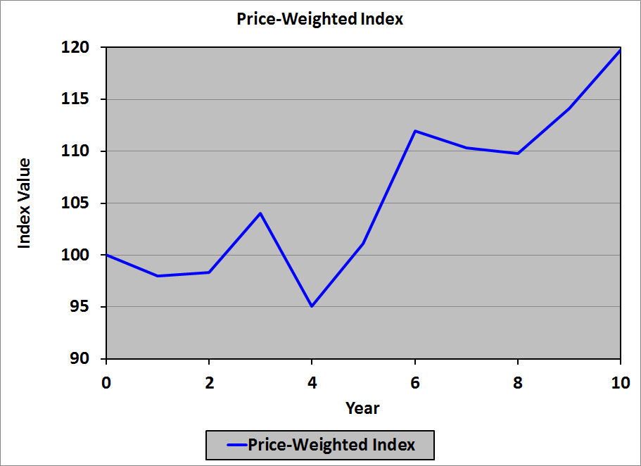
Here’s how the index value looks over time:

Price-Weighted Index Chart

Bias

Price-weighted indices are biased toward the stocks with the highest share price: a 1% change in a $100/share stock will have a much greater effect on the index than a 1% change in a $10/share stock.

Examples

The Dow Jones Industrial Average (DJIA) and the Nikkei index are price-weighted equity indices.

Issues in Constructing Tracking Portfolios

Because (the divisor for) a price-weighted index needs to be recalculated whenever a constituent stock undergoes a stock split, undergoes a reverse stock split, or issues a stock dividend, or is replaced by another company’s stock, a tracking portfolio will have to make adjustments for all of these events as well.  In particular, if a constituent stock undergoes a stock split or issues a stock dividend, a tracking portfolio will have more shares in that stock than in the other stocks and will therefore have to sell shares.  If a constituent stock undergoes a reverse stock split, a tracking portfolio will have fewer shares in that stock than in the other stocks and will therefore have to buy shares.  If one stock in the index is replaced with another stock, a tracking portfolio will have to sell all of its shares in the former and purchase the same number of shares in the latter.

Value-Weighted Indices

In a value-weighted index, the hypothetical portfolio contains all available shares of each stock.  There are two subcategories of value-weighted indices:

  • Unadjusted for free-float
  • Adjusted for free-float

Unadjusted for Free-Float

When a value-weighted index is not adjusted for free-float, the number of shares of each stock included in the index is the total number of shares issued and outstanding.  The formula to determine the value of the index at any time t is:

\[Value-Weighted\ Index_t\ =\ \left(\dfrac{\sum_{i=1}^nP_{i_t}Q_{i_t}}{\sum_{i=1}^nP_{i_b}Q_{i_b}}\right)\left(Beginning\ Index\ Value\right)\]

where:

  • \(n\): number of stocks in the index
  • \(P_{i_t}\): share price of stock i at time t
  • \(Q_{i_t}\): number of shares of stock i at time t
  • \(P_{i_b}\): share price of stock i outstanding at time b (beginning: when the index started)
  • \(Q_{i_b}\): number of shares of stock i outstanding at time b (beginning, when the index started)

The nice thing about value-weighted indices is that you don’t need to make any adjustments when there is a stock split, reverse stock split, or stock dividend: the total value of the outstanding stock doesn’t change when these events occur.

The divisor is the total market capitalization of all stocks in the index when the index originates.  Using our example data:

\begin{align}Divisor\ &=\ \sum_{i=1}^nP_{i_b}Q_{i_b}\\
\\
&=\ \$95.44\left(5,000,000\right)\ +\ \$22.37\left(20,000,000\right)\\
\\
&+\ \$44.21\left(10,000,000\right)\\
\\
&=\ \$1,366,700,000
\end{align}

The total market capitalization at each time is:

\begin{align}Time\ 0:\ \$95.44\ ×\ 5,000,000\ &+\ \$22.37\ ×\ 20,000,000\\
&+\ \$44.21\ ×\ 10,000,000\ =\ \$1,366,700,000\\
\\
Time\ 1:\ \$93.23\ ×\ 5,000,000\ &+\ \$20.43\ ×\ 20,000,000\\
&+\ \$45.08\ ×\ 10,000,000\ =\ \$1,325,550,000\\
\\
Time\ 2:\ \$92.96\ ×\ 5,000,000\ &+\ \$20.68\ ×\ 20,000,000\\
&+\ \$45.71\ ×\ 10,000,000\ =\ \$1,335,500,000\\
\\
Time\ 3:\ \$103.25\ ×\ 5,000,000\ &+\ \$19.68\ ×\ 20,000,000\\
&+\ \$45.57\ ×\ 10,000,000\ =\ \$1,365,550,000\\
\\
Time\ 4:\ \$90.29\ ×\ 5,000,000\ &+\ \$18.21\ ×\ 20,000,000\\
&+\ \$45.57\ ×\ 10,000,000\ =\ \$1,271,350,000\\
\\
Time\ 5:\ \$98.22\ ×\ 5,000,000\ &+\ \$19.64\ ×\ 20,000,000\\
&+\ \$45.99\ ×\ 10,000,000\ =\ \$1,343,800,000\\
\\
Time\ 6:\ \$59.45\ ×\ 10,000,000\ &+\ \$21.59\ ×\ 20,000,000\\
&+\ \$45.99\ ×\ 10,000,000\ =\ \$1,486,200,000\\
\\
Time\ 7:\ \$56.57\ ×\ 10,000,000\ &+\ \$22.59\ ×\ 20,000,000\\
&+\ \$45.99\ ×\ 10,000,000\ =\ \$1,477,400,000\\
\\
Time\ 8:\ \$55.83\ ×\ 10,000,000\ &+\ \$22.79\ ×\ 20,000,000\\
&+\ \$45.94\ ×\ 10,000,000\ =\ \$1,473,500,000\\
\\
Time\ 9:\ \$58.96\ ×\ 10,000,000\ &+\ \$24.42\ ×\ 20,000,000\\
&+\ \$46.12\ ×\ 10,000,000\ =\ \$1,539,200,000\\
\\
Time\ 10:\ \$64.62\ ×\ 10,000,000\ &+\ \$24.90\ ×\ 20,000,000\\
&+\ \$46.35\ ×\ 10,000,000\ =\ \$1,607,700,000\\
\end{align}

The corresponding index values are:

\begin{align}Time\ 0:\ \dfrac{\$1,366,700,000}{\$1,366,700,000}\ &=\ 100.00\\
\\
Time\ 1:\ \dfrac{\$1,325,550,000}{\$1,366,700,000}\ &=\ 96.99\\
\\
Time\ 2:\ \dfrac{\$1,335,500,000}{\$1,366,700,000}\ &=\ 97.72\\
\\
Time\ 3:\ \dfrac{\$1,365,550,000}{\$1,366,700,000}\ &=\ 99.92\\
\\
Time\ 4:\ \dfrac{\$1,271,350,000}{\$1,366,700,000}\ &=\ 93.02\\
\\
Time\ 5:\ \dfrac{\$1,343,800,000}{\$1,366,700,000}\ &=\ 98.32\\
\\
Time\ 6:\ \dfrac{\$1,486,200,000}{\$1,366,700,000}\ &=\ 108.74\\
\\
Time\ 7:\ \dfrac{\$1,477,400,000}{\$1,366,700,000}\ &=\ 108.10\\
\\
Time\ 8:\ \dfrac{\$1,473,500,000}{\$1,366,700,000}\ &=\ 107.81\\
\\
Time\ 9:\ \dfrac{\$1,539,200,000}{\$1,366,700,000}\ &=\ 112.62\\
\\
Time\ 10:\ \dfrac{\$1,607,700,000}{\$1,366,700,000}\ &=\ 117.63
\end{align}

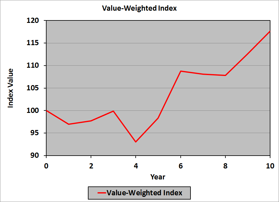
Here’s how the index value looks over time:

Value-Weighted Index Chart

Adjusted for Free-Float

Many companies have common shares which, although issued and outstanding, are not available to the general public for purchase.  One example of such shares would be those owned by the founders of the company, who have no intention of selling their shares.  Another example is corporate cross-holdings: two companies that are closely allied will purchase shares of each other, to demonstrate their solidarity; once again, these companies have no intention of selling their shares in each other.

The free-float adjustment recognizes these shares as being unavailable to the investing public: each company in a free-float adjusted, value-weighted index has an associated free-float factor (FFF): a number between zero and one that gives the percentage of outstanding shares that are available for the investing public to purchase.  The formula to determine the value of the free-float-adjusted index at any time t is:

\[Value-Weighted\ Index_t\ =\ \left(\dfrac{\sum_{i=1}^nP_{i_t}Q_{i_t}FFF_{i_t}}{\sum_{i=1}^nP_{i_b}Q_{i_b}FFF_{i_b}}\right)\left(Beginning\ Index\ Value\right)\]

where:

  • \(FFF_{i_t}\): free-float factor for stock i at time t
  • \(FFF_{i_b}\): free-float factor for stock i at time b

Bias

Value-weighted indices are biased toward the stocks with the highest market capitalization: a 1% change in a $100 million market cap stock will have a much greater effect on the index than a 1% change in a $10 million market cap stock.

Examples

The S&P 500, the NASDAQ, and the Wilshire 5000 indices are value-weighted equity indices.

Issues in Constructing Tracking Portfolios

Because a value-weighted index is not affected by stock splits, reverse stock splits, and stock dividends, a tracking portfolio will not have to make any adjustments for these events.  However, if one stock in the index is replaced with another stock, a tracking portfolio will have to sell all of its shares in the former and purchase an appropriate number of shares in the latter.

Equal-Weighted (or Unweighted) Indices

In an equal-weighted index, the hypothetical portfolio contains the same dollar (euro, yen, baht, pound, whatever) value of each stock; you can think of it as owning $1.00 worth of each (or €1.00 worth of each, or £1.00 worth of each, or . . . well . . . you get the idea).  The formula to determine the value of the index at any time t is:

\[Equal-Weighted\ Index_t\ =\ Index_{t-1}\left[1\ +\ \dfrac{\sum_{i=1}^n\left(\dfrac{P_{i_t}}{P_{i_{t-1}}}\ -\ 1\right)}{n}\right]\]

To understand the formula (which isn’t as difficult as it looks), note that \(\dfrac{P_{i_t}}{P_{i_{t-1}}}\ -\ 1\) is simply the return on stock i from time t − 1 to time t.  We sum those and divide by n to get the average return on all stocks from time t − 1 to time t.  We add that average return to 1 and multiply it by the previous index value: all we’ve done is increase the index value at time t − 1 by the average return.

Voilà!

The returns for each stock for year 1, and the average return for year 1, are computed as:

Stock A’s return:

\[\dfrac{\$93.23}{\$95.44}\ -\ 1\ =\ -2.32\%\]

Stock B’s return:

\[\dfrac{\$20.43}{\$22.37}\ -\ 1\ =\ -8.67\%\]

Stock C’s return:

\[\dfrac{\$45.08}{\$44.21}\ -\ 1\ =\ 1.97\%\]

Average return:

\[\dfrac{-2.32\%\ +\ -8.67\%\ +\ 1.97\%}{3}\ =\ -3.01\%\]

The returns for the constituent stocks for all of the years, and the corresponding average returns, are calculated similarly:

Year Stock A Stock B Stock C Return A Return B Return C Avg. Return
0 $95.44 $22.37 $44.21
1 $93.23 $20.43 $45.08 −2.32% −8.67% 1.97% −3.01%
2 $92.96 $20.68 $45.71 −0.29% 1.22% 1.40% 0.78%
3 $103.25 $19.68 $45.57 11.07% −4.84% −0.31% 1.98%
4 $90.29 $18.21 $45.57 −12.55% −7.47% 0.00% −6.67%
5 $98.22 $19.64 $45.99 8.78% 7.85% 0.92% 5.85%
6 $59.45 $21.59 $45.99 21.05%* 9.93% 0.00% 10.33%
7 $56.57 $22.59 $45.99 −4.84% 4.63% 0.00% −0.07%
8 $55.83 $22.79 $45.94 −1.31% 0.89% −0.11% −0.18%
9 $58.96 $24.42 $46.12 5.61% 7.15% 0.39% 4.38%
10 $64.62 $24.90 $46.35 9.60% 1.97% 0.50% 4.02%

*The year 6 return on stock A is calculated using $59.45 as the new price and $49.11 (= $98.22 / 2) as the old price, given the 2:1 split.

The corresponding index values are:

\begin{align}EWI_0\ &=\ 100.00\\
\\
EWI_1\ =\ 100.00\left(1\ +\ -3.01\%\right)\ &=\ 96.99\\
\\
EWI_2\ =\ 96.99\left(1\ +\ 0.78\%\right)\ &=\ 97.75\\
\\
EWI_3\ =\ 97.75\left(1\ +\ 1.98\%\right)\ &=\ 99.68\\
\\
EWI_4\ =\ 99.68\left(1\ +\ -6.67\%\right)\ &=\ 93.03\\
\\
EWI_5\ =\ 93.03\left(1\ +\ 5.85\%\right)\ &=\ 98.47\\
\\
EWI_6\ =\ 98.47\left(1\ +\ 10.33\%\right)\ &=\ 108.64\\
\\
EWI_7\ =\ 108.64\left(1\ +\ -0.07\%\right)\ &=\ 108.56\\
\\
EWI_8\ =\ 108.56\left(1\ +\ -0.18\%\right)\ &=\ 108.37\\
\\
EWI_9\ =\ 108.37\left(1\ +\ 4.38\%\right)\ &=\ 113.12\\
\\
EWI_{10}\ =\ 113.12\left(1\ +\ 4.02\%\right)\ &=\ 117.67\\
\end{align}

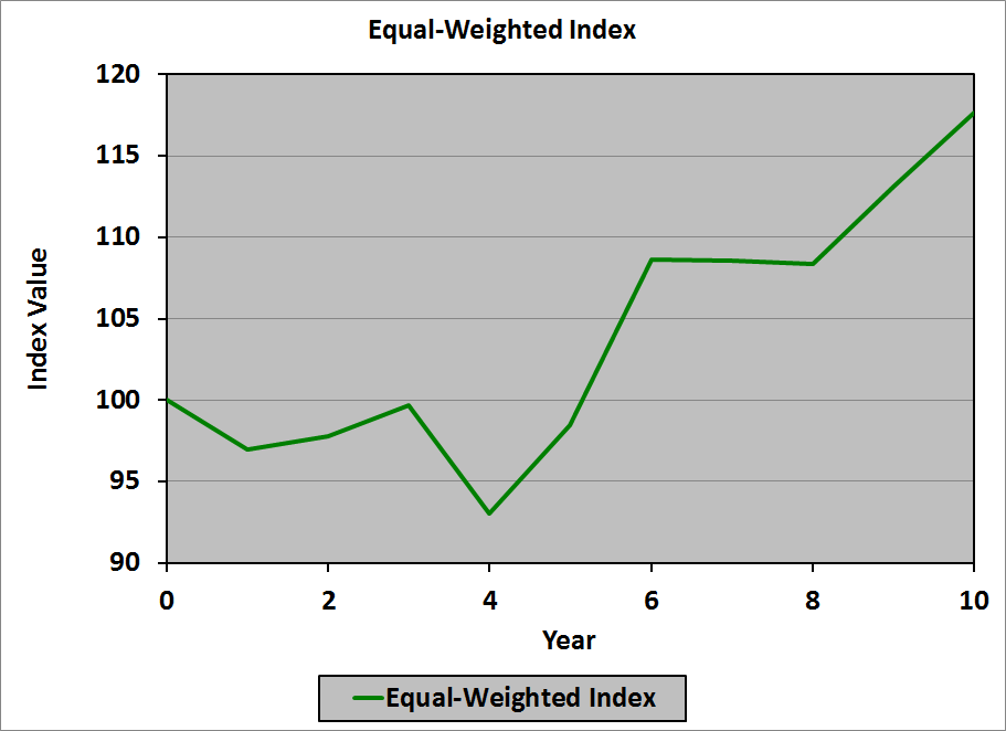
Here’s how the index value looks over time:

Equal-Weighted Index Chart

Bias

Equal-weighted indices are biased toward the stocks that have the highest volatility of returns.  Because small-cap stocks tend to have higher volatility of returns than large-cap stocks, equal-weighted indices tend to be biased toward the returns of small-cap stocks.

Examples

The Value Line Index and the Financial Times Ordinary Share Index are equal-weighted equity indices.

Issues in Constructing Tracking Portfolios

Because an equal-weighted index assumes the same value held in each stock, it is impractical to create a true tracking portfolio for such an index.  Every day the value of each security will change, so every day a tracking portfolio would have to rebalance back to equal weights, likely buying or selling fractions of shares of every stock it holds.   Apart from the impossibility of selling fractions of shares, transactions costs would be prohibitive.

As a practical approximation, therefore, portfolios that attempt to track equal-weighted indices rebalance much less frequently: usually quarterly.  Therefore, the weights on the securities in the portfolio will not be equal, so there will be differences in the performance of the portfolio and that of the index.

Oh, well.

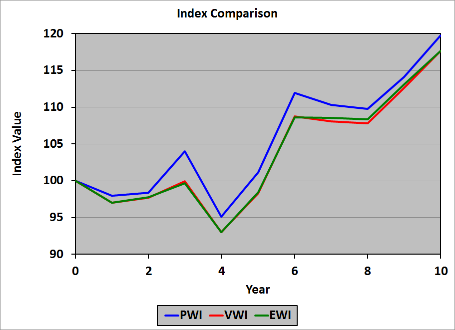
Comparison of Index Values

Here’s how the index values look over time:

Comparison of Indices Chart

Note that the strong influence of stock A (with the highest share price, even after the split) in the price-weighted index is quite evident in the comparison.

The price at which you will receive a margin call on a long position in a stock is given by:

\[margin\ call\ price\ =\ P_0\left(\frac{1\ –\ initial\ margin}{1\ –\ maintenance\ margin}\right)\]

where:

  • \(P_0\): initial price of the stock

The price at which you will receive a margin call on a short position in a stock is given by:

\[margin\ call\ price\ =\ P_0\left(\frac{1\ +\ initial\ margin}{1\ +\ maintenance\ margin}\right)\]

It might be useful to know how these formulae are derived, and, more importantly, why you do not need to know them.

How these Formulae are Derived

Let:

  • \(P_0\): initial price of the stock
  • \(P_m\): stock price that will generate a margin call
  • \(i\): initial margin
  • \(m\): maintenance margin

The initial margin that you have to post (in dollars) is:

\[P_0\ ×\ i\]

Long Position

When the price changes from \(P_0\) to \(P_m\), the price changes by an amount equal to \(P_m\ –\ P_0\). The value of the margin account for a long position changes by the same amount (e.g., if the price rises $5.00, the value of the margin account rises by $5.00), and becomes:

\[\left(P_0\ ×\ i\right)\ +\ \left(P_m\ –\ P_0\right)\]

At the margin call price, the value in the margin account will be the maintenance margin:

\[P_m\ ×\ m\]

Thus, at the margin call price,

\begin{align}\left(P_0\ ×\ i\right)\ +\ \left(P_m\ –\ P_0\right)\ &=\ P_m × m\\
\\
P_m\ –\ \left(P_m\ ×\ m\right)\ &=\ P_0\ –\ \left(P_0\ ×\ i\right)\\
\\
P_m\left(1\ –\ m\right)\ &=\ P_0\left(1\ –\ i\right)\\
\\
P_m\ &=\ P_0\left(\frac{1\ –\ i}{1\ –\ m}\right)
\end{align}

Short Position

When the price changes from \(P_0\) to \(P_m\), the value of the margin account for a short position becomes:

\[\left(P_0\ ×\ i\right)\ +\ \left(P_0\ –\ P_m\right)\]

and,

\begin{align}\left(P_0\ ×\ i\right)\ +\ \left(P_0\ –\ P_m\right)\ &=\ P_m × m\\
\\
P_m\ +\ \left(P_m\ ×\ m\right)\ &=\ P_0\ +\ \left(P_0\ ×\ i\right)\\
\\
P_m\left(1\ +\ m\right)\ &=\ P_0\left(1\ +\ i\right)\\
\\
P_m\ &=\ P_0\left(\frac{1\ +\ i}{1\ +\ m}\right)
\end{align}

Example

If the market price of a stock today is $25/share, the initial margin is 50% and the maintenance margin is 30%, then if you have a long position in the stock you will get a margin call if the price drops to:

\[$25\left(\frac{1\ –\ 0.5}{1\ –\ 0.3}\right)\ =\ $17.86\]

and if you have a short position in the stock you will get a margin call if the prices rises to:

\[$25\left(\frac{1\ +\ 0.5}{1\ +\ 0.3}\right)\ =\ $28.85\]

You can check these values to ensure that they make sense: your initial margin is $25.00 × 50% = $12.50.  If the price drops to $17.86 and you have a long position, your margin account is now $12.50 – ($25.00 – $17.86) = $5.36, and,

\[\frac{$5.36}{$17.36}\ =\ 0.30\]

If the price rises to $28.85 and you have a short position, your margin account is now $12.50 – ($28.85 – $25.00) = $8.65, and,

\[\frac{$8.65}{$28.85}\ =\ 0.30\]

Why You Don’t Need to Know These Formulae

Note, however, that you do not need to be able to calculate the price at which you will get a margin call; all you need to be able to do is check whether a given price is correct.  The reason is simple: on the exam, if you’re asked the price at which a margin call will occur, you know that one of the three answer choices given is correct; all you have to do is check one of them: the middle price (answer choice “b”).  Calculate the value of the margin account, and divide that by the price; if that’s the maintenance margin percentage, then “b” is the correct answer; if it’s not, you can deduce the correct answer.

For example, suppose that for the stock above you are asked to compute the price at which the long position would get a margin call, and the answer choices are:

  1. $17.86
  2. $18.50
  3. $20.00

You check answer choice “b”: the margin account value is $12.50 – ($25.00 – $18.50) = $6.00, and,

\[\frac{$6.00}{$18.50}\ =\ 0.323\]

This value is too big, so you know that answer “b” is incorrect, and you also know that the correct answer is smaller than $18.50, because at $18.50 the margin percentage is above the maintenance margin; thus, the price hasn’t fallen enough to drop the margin account to 30% of the price, so the correct answer has to be “a”.

There are a lot of formulae in the Level I CFA curriculum that you need to memorize, but if you can check the value of the margin account as shown here, you don’t need to memorize the formulae for the margin call price; save some room in your brain for the others you do need to memorize.