Financial Exam Help 123

To create a binomial interest rate tree, you need to start with:

1. A yield curve
2. An interest rate volatility

The yield curve can be a par curve, a spot curve, or a forward curve. (If you’re a bit fuzzy on the differences among these curves, look here.) For the remainder of this article, we’ll assume that we’re given a par curve; as we could generate the other curves given any one of them, it doesn’t really matter which one we get.

The interest rate volatility will be given as a standard deviation: σ. We’ll see in a moment how we use it to construct the tree.

The easiest way to explain how the tree is constructed is by going through an example, so here goes:

Suppose that the benchmark (annual pay) par curve is:

Maturity	Par Rate
1	2.00%
2	4.00%
3	5.60%
4	6.80%

The corresponding spot rates and (1-year) forward rates are:

Maturity	Spot Rate	Forward Rate
1	2.0000%	2.0000%
2	4.0408%	6.1224%
3	5.7333%	9.2014%
4	7.0587%	11.1355%

The (annual) interest rate volatility we’ll use for the tree will be σ = 10%. This is usually implemented as a continuous rate (though there’s no reason that it could not be an effective rate), meaning that we’ll be using a factor of e^σ = e^10% = 1.1052 to relate low and high interest rates at the same time in the tree.

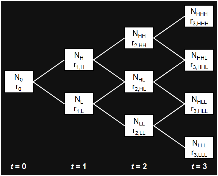
Here’s the tree we’ll be constructing:

For each node (i.e., white box), the N simply tells us which node it is: node zero (N₀), node low (N_L), node high (N_H), node low, low (N_LL), and so on; the r is the (1-year) forward rate at that node.

The keys to creating the binomial interest rate tree are that:

• The weights attached to each up leg and each down leg are all 50%. (Many people refer to these as probabilities, which is unfortunate. We’re not asserting anything about the likelihood of forward rates being higher or lower, we’re simply weighting the values we get in the upper leg and the lower leg. You’ll see.)
• All of the rates at a given time are related by the assumed volatility of interest rates.
• The tree has to give correct prices for (par) bonds.  This is known as calibrating the tree.

Although it’s trivial, for sake of completeness we’ll start at time t = 0, with r₀ at node N₀. The 1-year par bond pays a coupon of 2% ($20 on a $1,000 par bond), so discounting by r₀ has to give us par:

\begin{align}\$1,000 &= \frac{\$1,000 + \$20}{1 + r_0}\\
\\
\$1,000\left(1 + r_0\right) &= \$1,020\\
\\
\left(1 + r_0\right) &= \frac{\$1,020}{\$1,000} = 1.02\\
\\
r_0 &= 0.02\ =\ 2.00\%
\end{align}

So, not surprisingly, r₀ equals the 1-year forward rate starting today, which is the same as the 1-year spot rate, which is the same as the 1-year par rate.  Rest assured, it gets more exciting from here.

Moving to time t = 1, we have two rates to calculate: r_1,L at node N_L, and r_1,H at node N_H. We consider r_1,L to be one standard deviation down (1σ down) and r_1,H to be 1σ up from some sort of mean 1-year forward rate starting 1 year from today (think: up and down from the rate on the forward curve), so the relationship between r_1,L and r_1,H is that they differ by 2σ:

\[r_{1,H} = e^{2\sigma}r_{1,L} = e^{20\%}r_{1,L} = 1.2214r_{1,L}\]

The 2-year par bond pays a coupon of 4%, and discounting 50% (the upper weight) along the upper path and 50% (the lower weight) along the lower path (and remembering that we have a coupon payment at time t = 1, and that r₀ = 2%) has to give us par:

\begin{align}\$1,000 &= 0.5\left(\frac{\$1,040}{\left(1 + r_{1,H}\right)\left(1.02\right)} + \frac{$40}{1.02}\right)\\
\\
&+ 0.5\left(\frac{\$1,040}{\left(1 + r_{1,L}\right)\left(1.02\right)} + \frac{$40}{1.02}\right)\\
\\
\$1,000\left(1 + r_{1,H}\right)\left(1 + r_{1,L}\right)\left(1.02\right) &= \$520\left(1 + r_{1,L}\right) + \$520\left(1 + r_{1,H}\right)\\
\\
&+ \$40\left(1 + r_{1,L}\right)\left(1 + r_{1,H}\right)
\end{align}

Substituting r_1,H = 1.2214r_1,L gives:

\begin{align}\$1,020\left(1 + 1.2214r_{1,L}\right)\left(1 + r_{1,L}\right) &= \$520\left(1 + r_{1,L}\right)\\
\\
&+ \$520\left(1 + 1.2214r_{1,L}\right)\\
\\
&+ \$40\left(1 + r_{1,L}\right)\left(1 + 1.2214r_{1,L}\right)
\end{align}

Multiplying this all out and grouping the terms, we get:

\[\$1,196.97r_{1,L}^2 + \$1,021.85r_{1,L} – $60 = \$0\]

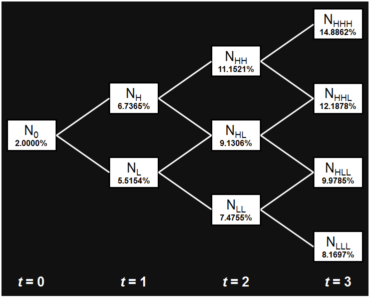
This is a quadratic equation in r_1,L which any high school algebra student could solve using the quadratic formula. (How exciting!) I’ll spare you the details and let you know that the solution that interests us is r_1,L = 5.5154%. Thus, r_1,H =1.2214(5.5154%) = 6.7365%.  (For whatever it’s worth, the other solution to the equation is r_1,L = −90.8844%.  It’s probably not the one we want to use.)  Note that in practice nobody would solve this equation; they use numerical methods (e.g., Excel’s Solver add-in) to approximate the solution.

If you compare these rates to the original forward curve, you’ll see that they look reasonable. The 1-year forward rate starting 1 year from today is 6.1224%. If you compare it to r_1,L and r_1,H, you get 6.1224% / 5.5153% = 1.1101, and 6.7364% / 6.1224% = 1.1003. Both of these are close to the factor of 1.1052 = e^10%, so we should be happy with the results.

Moving to time t = 2, we now have three rates to calculate: r_2,LL, r_2,HL, and r_2,HH. They’re related by r_2,HL = 1.2214r_2,LL and r_2,HH = 1.2214r_2,LL = 1.4918r_2,LL.  The 3-year par bond pays a coupon of 5.6%, and if we discount it along all of the paths (4 in total, each with a probability of 25% (= 0.5²)), we have to get par. If we follow a similar procedure to the one we used for t = 2, above, we will get a cubic (third-degree) equation for r_2,LL. This can be solved using Ferrari‘s formulae (though they were originally discovered by del Ferro and Tartaglia, and published by Cardano), but in practice, the solutions are found numerically. The solution that interests us is r_2,LL = 7.4755%, giving r_2,HL = 9.1306%, and r_2,HH = 11.1521%.

Again, if you compare these rates to the original forward curve (the 1-year forward rate starting 2 years from today is 9.2014%), you’ll see that they look reasonable: r_2,HL is very close to ₁f₂: 9.1306% vs. 9.2014%.

For time t = 4, we have four rates to calculate, we’re going to get a quartic (fourth-degree) equation for r_3,LLL, and we can solve it with Cardano‘s formulae (another of Ferrari‘s brainchildren published by Cardano). Once again, in practice the solutions will be found numerically: we’ll get r_3,LLL = 8.1697%, r_3,HLL = 9.9785%, r_3,HHL = 12.1878%, and r_3,HHH = 14.8862%.  Comparing these to the forward rate of 11.1355% makes them look reasonable.

Beyond time t = 4, we have no choice: we have to proceed numerically. (Abel (building on the work of Ruffini) – and, later, Galois – proved that there is no general algebraic solution to quintic (fifth-degree) and higher-order equations.)

The tree now looks like this:

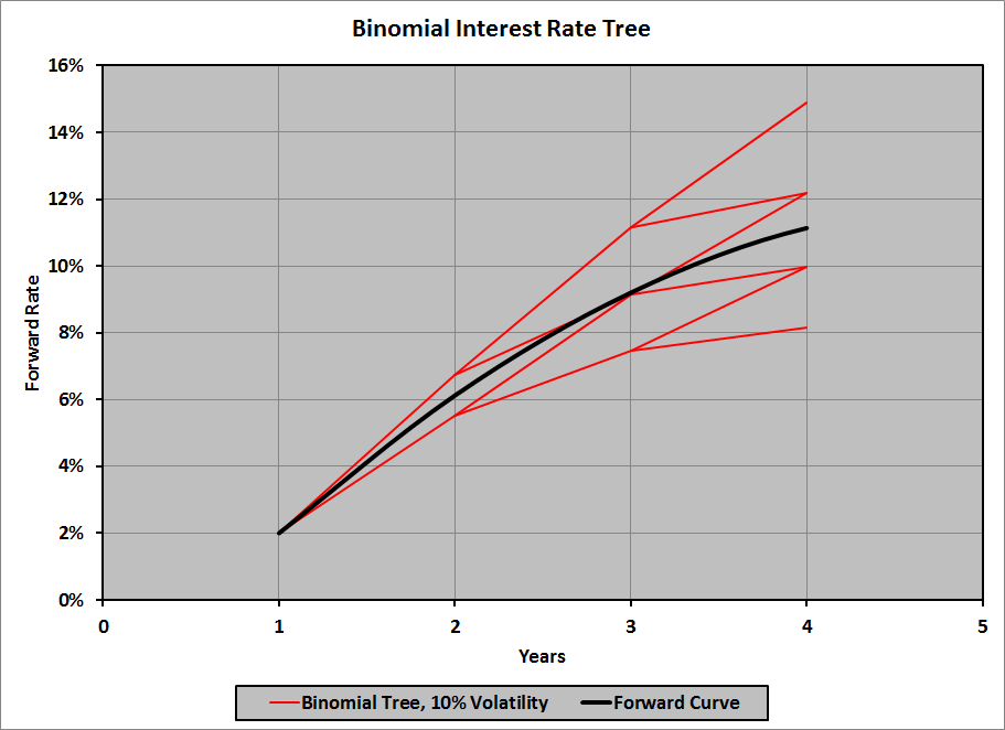
Graphically, here’s how the tree looks, compared to the forward curve:

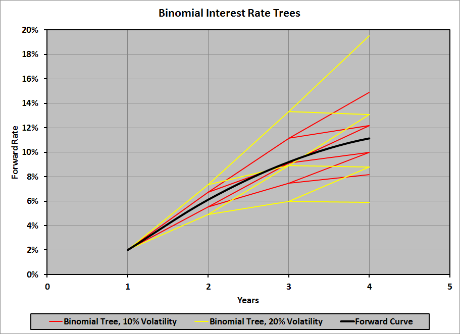
Here’s a comparison of the binomial tree with 10% interest rate volatility with one with 20% interest rate volatility:

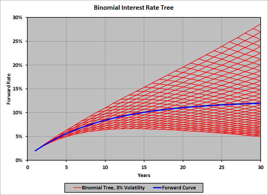
To get an idea of how big an impact interest rate volatility can have, here is a 30-year binomial interest rate tree with only 3% annual interest rate volatility; the maximum rate at 30 years is 28.6%:

At 5% annual volatility, the maximum rate at 30 years is 51.2%.  At 10% annual volatility, the maximum rate at 30 years is 218.1%!