What do we mean by “currency management“?
In a nutshell, we mean managing (i.e., adjusting) our exposure to changes in currency exchange rates. We might, for example,
- Hedge 100% (or as close to 100% as we can get) of our exposure to exchange rates (that exposure arising from existing investments in securities denominated in currencies other than our home currency)
- Hedge notably less than 100% of our exposure to exchange rates (from existing investments)
- Hedge notably more than 100% of our exposure to exchange rates (from existing investments)
- Invest actively in currencies (i.e., seek exposure to exchange rates) with no existing investments in securities denominated in those currencies
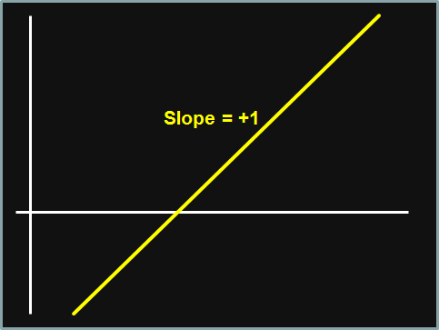
You can see that there is a continuum (or spectrum, which is more colorful) of currency exchange rate exposure, illustrated here:
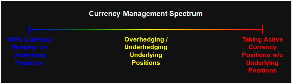
The blue (left) end of the spectrum is considered fully passive (conservative), while the red (right) end is considered fully active (liberal); in between can be considered a mix of active and passive (semi-active, or partially active, or moderate).
To explain currency management in its full, unabashed glory is more than I’d like to attempt in a single article, so this one will cover the basics while the companion article(s) will handle more of the heavy lifting.
CFA Institute’s Currency Exchange Rate Notation
CFA Institute has chosen to use a notation for currency exchange rates that is at odds with the common notation used in the financial industry. For example, if you were to go to Yahoo! Finance and look up the exchange rate between, say, USD and JPY, you would see this quote (as of the day that I’m writing this):
\[USD/JPY\ 136.42\]
This means that JPY 136.42 is equivalent (i.e., will buy you) USD 1.00. In this quote, USD is called the base currency and JPY is called the price currency.
Unfortunately, this is not the notation that CFA Institute uses. They would write the exchange rate as:
\[JPY/USD\ 136.42\]
where, once again, USD is the base currency and JPY is the price currency. I like to think of the base currency as a commodity (which, of course, it is), and I typically visualize it as oil; furthermore, when working problems, I will write it this way:
\[\frac{JPY\ 136.42}{USD\ 1.0}\]
I find that writing it that way ensures that I don’t make a silly mistake when I’m doing calculations (e.g., dividing by 136.42 when I should be multiplying by 136.42).
Note that this quote is equivalent to:
\[USD/JPY\ 0.007330\]
because
\[0.007330 = \frac{1}{136.42}\]
If, on the following day, the quote were:
\[JPY/USD\ 135.97\]
then the price of our “oil” (one USD, priced in JPY) has decreased. USD has depreciated relative to JPY, and, conversely, JPY has appreciated vis-à-vis USD. If we look at the new JPY/USD quote, it is:
\[USD/JPY\ 0.007355\]
If you deal in currency exchange in your daily work, you have my sympathies, because CFA Institute’s quoting convention will cause you no end of grief, especially when you’re under stress (as you may be when taking the exam). In many ways, it’s the same as visiting a country in which you have to drive on the side of the road that is opposite the side on which you drive at home. It feels very uncomfortable under the best of circumstances, and under stressful conditions (e.g., inclement weather, debris in the road, a traffic collision), can result in you instinctively choosing the wrong side, possibly with disastrous results. I wish you the best of luck. Sincerely.
The Scope of This Article
In this article I’ll cover:
- How currency markets work
- How currency exposure affects a portfolio’s performance
- How to measure currency exposure
- How to choose where on the currency management spectrum you should lie (hint: it has precious little to do with your favorite color; if it did, and your favorite color were purple, you’d be finished before you even started)
- What tools are available for currency management
- How those tools work
Here we go!
How Currency Markets Work
There are two currency markets about which we are concerned: the spot market and the forward market. In the spot market, the currencies are exchanged immediately (where “immediately” means two days after the trade date – quoted as “T + 2” – or, in some cases (notably CAD vs. USD), one day after the trade date (“T + 1”)); in the forward market, the currencies are exchanged at a time significantly in the future: 30, 60, 90 days after the transaction date.
Spot Markets & Spot Quotes
I’ve already covered CFA Institute’s odd (read: annoying) quoting convention, above. When the exchange rates are in the single digits – e.g., USD/CHF 1.0400, BRL*/EUR 5.4537, JPY/INR† 1.7392, and so on – they’re typically quoted to four decimal places, but when the exchange rates are in the triple digits – e.g., JPY/USD 136.07, ARS‡/EUR 130.89, ISK**/GBP 161.18 – they’re typically quoted to two decimal places. (I have no idea what’s typical for double-digit rates (e.g., INR/AUD 54.1346), or quadruple-or-more-digit rates (e.g., LAK††/NZD 9,477.36). On the exam, use whatever number of decimal places they give you.)
[*BRL = Brazilian real, †INR = Indian rupee, ‡ARS = Argentine peso, **ISK = Icelandic krona, ††LAK = Lao kip]
Currency dealers make their livings the same way that car dealers do: by buying at a lower price and selling at a higher price. Their adverts (quotations), therefore, show two prices:
- The bid price; i.e., the price they will pay (in the price currency) if they’re buying a particular base currency
- The ask (or offer) price: i.e., the price they will charge you (in the price currency) if they’re selling that same base currency
The bid price is always listed first, the ask price, second. A typical published spot market quote (with USD as the base currency and EUR as the price currency) might be:
\[EUR/USD\ 0.9424/0.9494\]
Here, the bid rate is:
\[EUR/USD\ 0.9424\]
and the ask rate is:
\[EUR/USD\ 0.9494\]
For example, if you wanted to sell USD 1 million to this dealer (for EUR), you would receive:
\[USD\ 1,000,000\ \left(EUR/USD\ 0.9424\right) = EUR\ 942,400\]
If you wanted to buy USD 1 million from this dealer (for EUR), you would pay:
\[USD\ 1,000,000\ \left(EUR/USD\ 0.9494\right) = EUR\ 949,400\]
If EUR were the base currency and USD the price currency, then the quote would be:
\[USD/EUR\ 1.0533/1.0611\]
Note that:
\[1.0533 = \frac{1}{0.9494}\]
and:
\[1.0611 = \frac{1}{0.9424}\]
Forward Markets & Forward Quotes
The quotes for forward exchange rates are generally given relative to the corresponding spot rates, and are generally quoted in points, where one point is the rightmost digit (the least significant digit, as mathematicians would say) in the spot quote. So, for exchange rates quoted to four decimal places, one point is 1/10,000 (= 0.0001) of the price currency; for exchange rates quoted to two decimal places, one point is 1/100 (= 0.01) of the price currency. Note that forward points are often quoted to one decimal place, so the corresponding forward quotes have one decimal place more than the spot rate. A typical quote showing the spot rates and the forward points might be:
| EUR/USD |
| Maturity |
Spot Rate or Forward Points |
| Spot |
0.9424 / 0.9494 |
| 1 month |
−13.3 / −13.4 |
| 3 months |
−47.0 / −47.3 |
| 6 months |
−115.6 / −116.5 |
| 12 months |
−215.9 / −217.5 |
Thus, the 1-month forward bid rate is:
\[EUR/USD\ 0.9424 + \left(\frac{-13.3}{10,000}\right) = EUR/USD\ 0.94107\]
the 1-month forward ask rate is:
\[EUR/USD\ 0.9494 + \left(\frac{-13.4}{10,000}\right) = EUR/USD\ 0.94806\]
and so on.
On the exam, they will generally tell you how big one point is (often in a footnote to a table such as the one above), so be on the lookout for that.
How Currency Exposure Affects a Portfolio’s Performance
Effect on Returns
Investors are interested in the returns they earn in their portfolios, with those returns measured in their home currency. Therefore, to measure an investment’s performance it isn’t sufficient to calculate the return in the currency in which that investment is denominated; you have to measure the return in the investor’s home currency. (Of course, this means that the same investment may have a different return for one investor than for another, if those investors’ home currencies differ from each other.)
Imagine that we have two investors:
- Investor E’s home currency is EUR
- Investor J’s home currency is JPY
Each of these investors buys 1,000 shares of WI stock (an Australian company) on 23 June 2022 and sells those shares on 23 June 2023. We’ll calculate the return to each of these investors in their respective home currencies. The common data for these investors is that they buy the stock when its price is AUD 47.55 per share, and sell it one year later when its price is AUD 51.25 per share. The unique data for each investor are:
- Investor E
- Beginning exchange rate: EUR/AUD 0.6560
- Ending exchange rate: EUR/AUD 0.6725
- Investor J
- Beginning exchange rate: JPY/AUD 93.14
- Ending exchange rate: JPY/AUD 90.22
Let’s walk through the transactions for each investor:
- Investor E
- 23 June 2022: buy 1,000 shares of WI. The total investment is AUD 47,550, or EUR 31,193 (= AUD 47,550 × EUR/AUD 0.6560)
- 23 June 2023: sell 1,000 shares of WI. The total proceeds are AUD 51,250, or EUR 34,466 (= AUD 47,550 × EUR/AUD 0.6725)
- The profit is EUR 3,273, or 10.4922% (= EUR 3,273 / EUR 31,193)
- Investor J
- 23 June 2022: buy 1,000 shares of WI. The total investment is AUD 47,550, or JPY 4,428,807 (= AUD 47,550 × JPY/AUD 93.14)
- 23 June 2023: sell 1,000 shares of WI. The total proceeds are AUD 51,250, or JPY 4,623,775 (= AUD 47,550 × EUR/AUD 90.22)
- The profit is JPY 194,968, or 4.4023% (= JPY 194,968 / JPY 4,428,807)
Each investor bought 1,000 shares of WI at AUD 47.55 and sold them at AUD 51.25, for a profit of AUD 3,700, or 7.7813% (= AUD 3,700 / AUD 47,550). How, then, did investor J’s performance lag investor E’s performance? In a word, exchange rates. (OK, that’s two words. Sue me.)
Investor E bought AUD for EUR/AUD 0.6560 and sold them one year later for EUR/AUD 0.6725. The return on the exchange rate was EUR/AUD 0.0165, or 2.5152% (= EUR/AUD 0.0165 / EUR/AUD 0.6560). Investor J bought AUD for JPY/AUD 93.14 and sold them one year later for JPY/AUD 90.22. The return on the exchange rate was JPY/AUD −2.92, or −3.1351% (= JPY/AUD −2.92 / JPY/AUD 93.14).
The return in domestic currency on an investment denominated in another currency comprises two returns (which are compounded):
- The investment’s return in its own (local) currency
- The return on the currency exchange rate
For investor E, we have:
\begin{align}1 + return_{EUR} &= \left(1 + return_{AUD}\right)\left(1 + return_{EUR/AUD}\right)\\
\\
&= \left(1 + 7.7813\%\right)\left(1 + 2.5152\%\right) = 1.104922\\
\\
return_{EUR} &= 0.104922 = 10.4922\%
\end{align}
For investor J, we have:
\begin{align}1 + return_{JPY} &= \left(1 + return_{AUD}\right)\left(1 + return_{JPY/AUD}\right)\\
\\
&= \left(1 + 7.7813\%\right)\left(1 + -3.1351\%\right) = 1.044022\\
\\
return_{JPY} &= 0.044022 = 4.4022\%
\end{align}
(There’s a slight discrepancy from rounding; pay it no heed.)
Therefore, unless an investor can hedge the exchange rate completely, or unless the exchange rate cannot change (i.e., the investment’s local currency is pegged to the investor’s home currency), the return in the investor’s home currency will be different from the return in the investment’s local currency. It might be higher (if the investment’s local currency appreciates vis-à-vis the investor’s home currency), or it might be lower (if the investment’s local currency depreciates vis-à-vis the investor’s home currency). Note that in the example above, AUD appreciated versus EUR and depreciated versus JPY; the investor E’s return was higher than the AUD return while the investor J’s return was lower than the AUD return.
A word of caution: the exchange rate (i.e., currency) returns have to be calculated with the investment’s currency as the base currency and the investor’s home currency as the price currency, as I did above. If the exchange rate quotes were given as AUD/EUR or AUD/JPY, you would have to convert them to EUR/AUD or JPY/AUD before computing the currency returns.
Sometimes the curriculum offers an approximation; for example:
\[return_{EUR} ≈ return_{AUD} + return_{EUR/AUD}\]
In words: the return in the investor’s home currency is approximately the return in the investment’s local currency plus the currency return. As I say, this is an approximation, but it may get you close enough to the correct answer that you needn’t do the compounding. Personally, I’d do the compounding.
Effect on Risk
The effect that currency exchange rates have on the risk of an investment is complicated. I’ll describe the simplification that the curriculum uses, but please bear in mind that it’s a simplification; the real effect is more difficult to analyze.
Properly, given the return on the investment in its local currency (\(r_{LC}\)) and the return on the foreign currency exchange rate (\(r_{FX}\)), the return on the investment in the investor’s home (domestic) currency is given by:
\begin{align}1 + r_{DC} &= \left(1 + r_{LC}\right)\left(1 + r_{FX}\right)\\
\\
r_{DC} &= \left(1 + r_{LC}\right)\left(1 + r_{FX}\right) – 1\\
\\
&= 1 + r_{LC} + r_{FX} + \left(r_{LC}\right)\left(r_{FX}\right) – 1\\
\\
&= r_{LC} + r_{FX} + \left(r_{LC}\right)\left(r_{FX}\right)
\end{align}
As a simplification, we choose to ignore the last term (which will be significantly smaller than the others), so we’ll use:
\[r_{DC} ≈ r_{LC} + r_{FX}\]
In essence, we’re looking at our investment as a portfolio having two sources of return (or two assets), each with a weight of 100% (I’ll get to why they each have a weight of 100% in a moment; have faith):
- The foreign investment
- The foreign currency
You’ll recall from Level I that when you have a portfolio with two assets, \(A\) and \(B\), with weights, respectively, \(w_A\) and \(w_B\), and returns, respectively, \(r_A\) and \(r_B\), then the variance of returns for the portfolio is given by:
\begin{align}σ^2_{r_{port}} &= w^2_Aσ^2_{r_A} + w^2_Bσ^2_{r_B} + 2w_Aw_Bσ_{r_B}σ_{r_A}ρ_{r_A,r_B}\\
\\
&= w^2_Aσ^2_{r_A} + w^2_Bσ^2_{r_B} + 2w_Aw_BCOV\left(r_A,r_B\right)
\end{align}
For our portfolio, we use the same formula, noting that the weights are each 100%:
\begin{align}σ^2_{r_{DC}} &≈ w^2_{LC}σ^2_{r_{LC}} + w^2_{FX}σ^2_{r_{FX}} + 2w_{LC}w_{FX}σ_{r_{LC}}σ_{r_{FX}}ρ_{r_{LC},r_{FX}}\\
\\
&= σ^2_{r_{LC}} + σ^2_{r_{FX}} + 2σ_{r_{LC}}σ_{r_{FX}}ρ_{r_{LC},r_{FX}}\\
\\
&= σ^2_{r_{LC}} + σ^2_{r_{FX}} + 2COV\left(r_{LC},r_{FX}\right)
\end{align}
What we get from these formulae is that if the correlation of the investment’s returns (in its local currency) and the exchange rate returns is zero or positive, the variance of returns in the (investor’s) domestic currency will be higher than the variance of returns in the local currency. If the correlation is negative and big enough (in absolute value), then the variance of returns in the domestic currency can be lower than the variance of returns in the local currency. So, with a negative correlation of LC and FX returns, there can be a diversification benefit to retaining the exposure to the currency exchange rate. As always, you need to look at the returns carefully to determine how large that benefit will be, and you may need to consider a tradeoff between possibly higher expected returns and possibly higher expected risk.
Why Are The Weights Both 100%? That Seems Weird
Think of a normal (domestic investments only) portfolio such as you had at Level I or Level II: say, 60% GOOG and 40% AAPL (for a USD-based investor). In that portfolio, 60% of your portfolio value would be subject to the return on GOOG, and 40% of your portfolio value would be subject to the return on AAPL: those returns run in parallel (side-by-side). When we calculate the variance of that portfolio’s returns, we use a weight of 0.6 (= 60%) for the GOOG returns and a weight of 0.4 (= 40%) for the AAPL returns. Easy-peasy.
Now, consider a (Level III) portfolio holding, say, an AUD-denominated stock for, say, a USD-based investor. Because 100% of the portfolio is invested in the stock, the weight on the stock’s return (in AUD) is 1.0 (= 100%). And because 100% of the AUD investment will be subject to the return on the USD/AUD exchange rate, the weight on the currency return is also 1.0 (= 100%). Unlike the Level I / Level II portfolio example, the returns in the Level III portfolio run in series (one after the other), not in parallel. It’s similar to a parlay at the racetrack.
Example
Suppose that the (annual) standard deviation of the AUD investment’s returns in local currency is 4.5%, the standard deviation of the EUR/AUD exchange rate return is 2.7%, and the correlation of the local currency (i.e., AUD) return and the EUR/AUD exchange rate return is −0.20. Then the volatility of returns in EUR is (approximately):
\begin{align}σ^2_{r_{EUR}} &≈ σ^2_{r_{AUD}} + σ^2_{r_{EUR/AUD}} + 2σ_{r_{AUD}}σ_{r_{EUR/AUD}}ρ_{r_{AUD},r_{EUR/AUD}}\\
\\
&= \left(4.5\%\right)^2 + \left(2.7\%\right)^2 + 2\left(4.5\%\right)\left(2.7\%\right)\left(-0.20\right)\\
\\
&= 0.002688\\
\\
σ_{r_{EUR}} &= \sqrt{0.002688} = 0.047624 = 4.7624\%
\end{align}
By retaining the EUR/AUD exchange rate exposure, investor E will earn a significantly higher return (10.4922% vs. 7.7813%) with somewhat higher risk (4.7624% vs. 4.50%). Investor E will have to decide whether the extra return is worth the extra risk.
Suppose further that the standard deviation of the JPY/AUD exchange rate is 3.9%, and the correlation of the AUD return and the JPY/AUD exchange rate return is +0.30. Then the volatility of returns in JPY is (approximately):
\begin{align}σ^2_{r_{JPY}} &≈ σ^2_{r_{AUD}} + σ^2_{r_{JPY/AUD}} + 2σ_{r_{AUD}}σ_{r_{JPY/AUD}}ρ_{r_{AUD},r_{JPY/AUD}}\\
\\
&= \left(4.5\%\right)^2 + \left(3.9\%\right)^2 + 2\left(4.5\%\right)\left(3.9\%\right)\left(0.30\right)\\
\\
&= 0.004599\\
\\
σ_{r_{JPY}} &= \sqrt{0.004599} = 0.067816 = 6.7816\%
\end{align}
By retaining the JPY/AUD exchange rate exposure, investor J will earn a significantly lower return (4.4023% vs. 7.7813%) with significantly higher risk (6.7816% vs. 4.50%). Investor J should probably decide to hedge the JPY/AUD exchange rate risk.
How to Measure Currency Exposure
Measuring currency exposure should be a simple matter, but I have found that candidates occasionally get confused about long vs. short exposure.
In my view, the easiest way to keep it straight is to think about what you will do at the end to close out your position. Forgetting about foreign currencies for a moment, imagine that you own bond L (which you would call a long position in bond L) and that you issued bond S (a short position in bond S). To close out the long position, you will sell bond L; to close out the short position, you will buy bond S. In general,
- A long position is one which you close out by selling the underlying
- A short position is one which you close out by buying the underlying
So it is with currency positions. Suppose that you’re an investor whose home currency is CHF (Swiss francs), and you buy a stock denominated in ARS (Argentine pesos). You’re long the stock, of course, and you’re also long ARS: to close out the position you will sell the stock (long the stock) and receive ARS, then sell the ARS (hence, long ARS) and receive CHF. If you borrowed HKD (Hong Kong dollars), then you’re short HKD; to close the position you’ll have to buy HKD (hence, short HKD), paying CHF, then deliver the HKD to the lender to pay off the loan.
Another way to think about long and short positions is to see what happens to the value of your portfolio when the value of the position increases. In general,
- If you’re long an asset and its value increases, the value of your portfolio increases
- If you’re short an asset and its value increases, the value of your portfolio decreases
Thus, if your home currency is CHF and you’re long ARS, then the value of your portfolio increases when the value of ARS increases (i.e., the CHF/ARS exchange rate increases; ARS appreciates vis-à-vis CHF). If you’re short HKD, then the value of your portfolio decreases when the value of HKD increases (i.e., the CHF/HKD exchange rate increases, HKD appreciates vis-à-vis CHF).
And, conversely, if you’re long a currency that depreciates, the value of your portfolio decreases, and if you’re short a currency that depreciates, the value of your portfolio increases.
How to Choose Where on the Currency Management Spectrum a Portfolio Should Lie
Where on the currency management spectrum a portfolio should lie depends largely on the risk tolerance of the owner, as well as the specifics of the portfolio’s investment policy statement (IPS). However, within those broad categories there are specifics that may suggest a more passive or a more active currency management approach.
Generalities
Risk Tolerance
In general, the lower an investor’s risk tolerance, the more passive (conservative) the currency management strategy you should employ. At the extreme, this would suggest hedging 100% of currency risk exposure (to the extent that that is possible). The higher the investor’s risk tolerance, the more active (liberal) the currency management strategy can be. At the extreme, you can treat currencies as a separate asset class and take active positions (long or short) in currencies without having positions in any underlying investments denominated in those currencies.
Investment Policy Statement (IPS)
A portfolio’s IPS will often (indeed, should) lay out the objectives and constraints on currency management. Amongst the topics that an IPS might cover in this regard are:
- Limits on the specific currencies to which the portfolio can be exposed
- Limits on the amount and types of investments denominated in foreign currencies
- Limits on the level of currency exchange rate hedging (either allowable limits, or required limits)
- Limits on the types of derivatives that may be used to hedge currency exchange rate exposure
- Minimum frequency for rebalancing currency hedges
Fewer allowable currency exposures, lower limits on the amounts of investments denominated in foreign currencies, tighter limits (around 100%) on the level of currency exchange rate hedging, and more frequent rebalancing all point toward a more passive currency management strategy, while more allowable currency exposures, higher limits on amounts of foreign investments, looser limits on hedging, and less frequent rebalancing argue for a more active strategy.
Specifics
Specific situations that argue for a more passive (conservative) currency management strategy include:
- Shorter term portfolio investment objectives
- Investors (beneficial owners of the portfolio) who do not experience ex post regret (i.e., who put on the brave face) over missed opportunities
- Higher immediate income/liquidity needs of the portfolio
- A higher percentage of foreign currency fixed-income assets than equity assets
- Inexpensive, readily available currency hedging tools
- Volatile financial markets
- Investors (beneficial owners of the portfolio) or portfolio managers who are skeptical of the expected benefits of active currency management
Specific situations that argue for a more active (liberal) currency management strategy include:
- Longer term portfolio investment objectives
- Investors (beneficial owners of the portfolio) who experience ex post regret over (i.e., who whine about) missed opportunities
- Lower immediate income/liquidity needs of the portfolio
- A higher percentage of foreign currency equity assets than fixed-income assets
- Expensive, or limited currency hedging tools
- Stable financial markets
- Investors (beneficial owners of the portfolio) or portfolio managers who believe in the expected benefits of active currency management
Why? (That Is: Why Do Each Of These Situations Argue For What I Suggest?)
- Length of the term of portfolio objectives
The general thinking is that over the long run, currency exchange rate returns are near zero, but that in the short run they may be significantly different from zero: either positive or else negative. Therefore, long-term objectives suggest not hedging exchange rate risk (a useless expense), while short-term objectives suggest hedging.
If investors are likely to whine about missing an opportunity to have benefited from a favorable exchange rate movement, then hedging the exchange rate will likely vex them. If they’re not likely to whine about it, then hedging it will go unnoticed.
If a portfolio has specific income or liquidity needs, then it is better for the return in its home currency to be stable; this argues for hedging the exchange rate, especially when the investment is in fixed income.
Fixed-income investments are strongly affected by local interest rates, as are exchange rates (and in the same direction). Equity investment are less strongly affected by local interest rates. Therefore, the volatility of returns (in the investor’s home currency) of fixed-income investments tends to be higher than the volatility of returns (in the investor’s home currency) of equity investments.
- Expensive or limited currency hedging tools
This one’s easy: is it’s expensive or impossible to hedge currency risk, then you’ll leave it unhedged (which is an active strategy). If it’s not expensive or impossible to hedge, you’re more likely to hedge 100%.
- Volatile vs. stable financial markets
Another easy one: if financial markets (i.e., exchange rates) are volatile, there’s more incentive to hedge 100%; if they’re stable, there’s less incentive to hedge (why spend the money when they’re not going to change anyway?).
- Belief in the benefits of active currency management
The third easy one: if you believe in the benefits of active currency management, be active; if not, be passive.
A Note on Hedging
For a fully passive (conservative) currency management program, an investor would need to hedge each currency exchange rate to which their portfolio is exposed 100%; i.e., for every foreign currency cash flow that they will receive or pay, they need to lock in the currency exchange rate. This requires that the investor know both the amount of each cash flow and the timing of each cash flow, with certainty.
For the most part, this is impossible.
An investor who buys foreign, risk-free, fixed rate bonds and intends to hold those bonds to maturity can, theoretically, hedge their exchange rate exposure 100%: they know the amount and timing of the coupon and par payments, so they can hedge each of those payments completely. The only problems they may experience would be the (theoretically extremely rare) possibility of a default, and the possibility that they may change their mind and decide to sell the bond before maturity.
However, for virtually any other investment, 100% hedging is impossible. If the investor buys a bond but does not intend to hold it to maturity, the investor knows neither the amount nor the timing of the final cash flow (when they sell the bond). If the investor buys a risky bond, then they do no know for certain when (or whether) they will receive coupon payments, let alone the final payment when the bond matures (or they sell it). If an investor buys a stock, they cannot know when they will sell the stock, nor what its share price will be when they do.
In these circumstances, a common practice is to hedge the original investment amount, and perhaps adjust the hedge up or down in the future as the value of the investment increases or decreases, respectively. It’s not perfect, but it’s reasonable.
Currency Management Tools
Currency management is generally implemented with derivatives: futures, forwards, options, and swaps. I’ll list the main types of tools in this section, then describe how they work in the next section.
The main types of currency management tools are:
- Currency futures contracts
- Agreements to exchange a specific amount of one currency for a specific amount of another currency on a specific date; the counterparty is the clearinghouse
- Currency forward contracts
- Agreements to exchange a specific amount of one currency for a specific amount of another currency on a specific date; the counterparty is another investor (typically a large financial institution)
- Currency options
- Call options
- The right to buy a specific amount of one currency by paying a specific amount of another currency on (or, possibly, before) a specific date
- May be exchange-traded (standardized) or over-the-counter (custom)
- Put options
- The right to sell a specific amount of one currency by receiving a specific amount of another currency on (or, possibly, before) a specific date
- May be exchange-traded (standardized) or over-the-counter (custom)
- Exotic options
- Knock-in options
- Knock-out options
- Digital options
- Currency swaps
- Fixed-for-fixed
- Fixed-for-floating
- Floating-for-floating
How Currency Management Tools Work
Currency Futures and Forward Contracts
A currency futures (or currency forward) contract is an agreement to exchange a given amount of one currency for an given amount of another currency at a specified date in the future; e.g., in 30 days, 60 days, 120 days, or 360 days. Fundamentally, currency futures and currency forwards are the same thing, they differ only in some details of implementation. For example,
- Currency futures contracts trade on exchanges, whereas currency forwards do not
- Currency futures contracts are standardized (currencies, amounts, maturities, delivery dates, and so on), whereas currency forwards are custom contracts
- In currency futures contracts the counterparty is always the clearinghouse (which is assumed to have no default risk), whereas in currency forward contracts the counterparty is another investor (typically an institutional investor, such as a bank)
- Currency futures contracts typically require you to post a margin, whereas currency forward contracts typically do not require a margin
- Currency futures contracts are typically marked to market daily (or, possibly, more frequently if markets are volatile), with any gain credited to or any loss deducted from the margin account, whereas currency forward contracts typically are not marked to market
For our purposes, these two types of contracts accomplish the same goal, so from now on I’ll refer to them simply as forwards.
The long/short positions in a currency forward contract are determined relative to the base currency:
- The long position is buying (receiving) the base currency and selling (delivering) the price currency
- The short position is selling (delivering) the base currency and buying (receiving) the price currency
Thus, the long position in a forward contract on, say, the INR/GBP (Indian rupee / British pound) exchange rate is equivalent to the short position in a forward contract on GBP/INR, and the short position in a forward on INR/GBP is equivalent to the long position in a forward on GBP/INR.
The exchange rate on a currency forward contract (which is known as the price of the forward) is determined using the spot exchange rate (at the inception of the forward) and interest rate parity (using the risk-free interest rates for the two currencies involved). For example, suppose that investor S, whose home currency is SEK (Swedish krona), has a long position in a stock denominated in NZD (New Zealand dollars). The spot exchange rate is SEK/NZD 6.3744. Investor S wants to hedge the SEK/NZD exchange rate for 6 months. The 6-month SEK risk-free rate is 1.793% (nominal, compounded semiannually), and the 6-month NZD risk-free rate is 3.494%. The 6-month SEK/NZD forward rate is therefore:
\[SEK/NZD\ 6.3744\left(\frac{1 + \dfrac{1.793\%}{2}}{1 + \dfrac{3.494\%}{2}}\right) = SEK/NZD\ 6.3211\]
Therefore, investor S will enter into a 6-month forward contract to deliver (some amount of) NZD and receive SEK, with an agreed exchange rate of SEK/NZD 6.3211.
In practice, there won’t be a single SEK/NZD spot rate or a single SEK/NZD 6-month forward rate; there will be a bid rate and an ask rate for each. The spot rate might be quoted as SEK/NZD 6.3266/6.4222 with the forward points quoted as −529.0/−537.0. Because Investor S will be selling NZD in the future, she will use the spot bid rate plus the bid points, giving an all-in forward rate of:
\[SEK/NZD\ 6.3266 + \frac{-529}{10,000} = SEK/NZD\ 6.2737\]
A currency forward contract has an advantage and a disadvantage. The advantage is that if the exchange rate moves unfavorably (in the above example, SEK/NZD decreases below the agreed forward rate), the investor will not lose any money, as the counterparty is obligated to settle the contract at the agreed (higher) exchange rate. The disadvantage is that if the exchange rate moves favorably (in the above example, SEK/NZD increases above the agreed forward rate), the investor will not gain any money, as the counterparty is, once again, obligated to settle the contract at the agreed (in this case, lower) exchange rate.
Currency Options
First, a bit about terminology. In the world of options, we tend to talk about prices: the strike price (and, for barrier options, the barrier price; see Exotic Options, below). For currencies, we should be talking about rates: exchange rates. But to keep the terminology consistent with what’s used in practice, I’ll stick with price. Thus, I’ll write “spot price” when I mean “spot rate”, or “strike price” when I mean “strike rate”. If you bear in mind that prices of currencies are simply exchange rates, you’ll be fine.
And, just to make it a little more complex, the price of an option is just that: the price (or premium) you pay to buy the option. You’ll recognize that one easily because it won’t be preceded immediately by “spot”, “strike”, or “barrier”.
Sigh.
(Vanilla) Call Options and Put Options
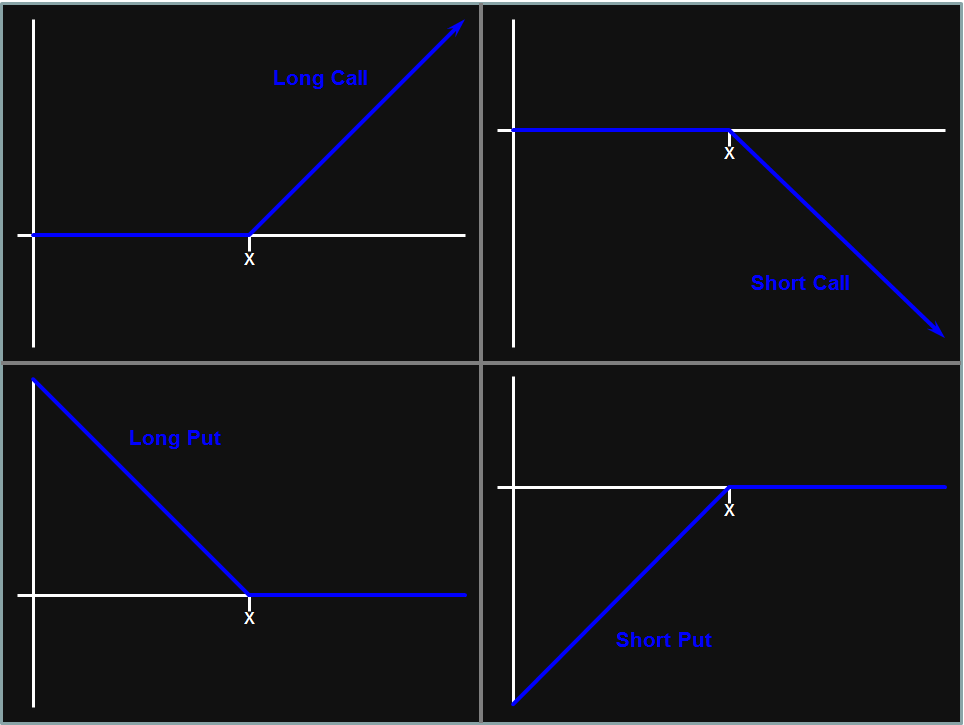
A currency call option gives the owner (the long position) the right (but not the obligation) to purchase a given amount of the base currency for a given amount of the price currency (i.e., at a given exchange rate, the strike rate, or strike price). If the option is European, the owner can exercise it only at expiry. If the option is American, the owner can exercise it anytime at or before expiry. (There are also Bermuda currency call options, Canary currency call options, and other more exotic types of call options, but we’ll stick with European and American here.) A currency put option gives the owner the right (but not the obligation) to sell a given amount of the base currency for a given amount of the price currency (i.e., at a given exchange rate, the strike rate, or strike price). Again, these can be European, or American, or something more exotic.)
Because the position is relative to the base currency, a call option on, say, the INR/GBP exchange rate is equivalent to a put option on GBP/INR, and a put option on INR/GBP is equivalent to a call option on GBP/INR. Note, too, that a short position in any of these options does obligate the investor if the owner (the long position) should choose to exercise the option.
The price of a currency call option or put option is the premium that one has to pay upfront to purchase the option. Determining a fair price for currency options is more difficult than for stock options (for which the Black-Scholes-Merton model gives an explicit formula for the option price) because there are two risk-free interest rates involved, and because those interest rates directly affect the value of the exchange rate (as opposed to being only discount rates to determine the present value). Therefore, I will not discuss in detail the pricing of currency options.
As with options on other underlying assets (stocks, bonds, commodities, and so on), the price of a currency option has both an intrinsic value and a time value. The intrinsic value is the value of the option if it were to expire today; it would be positive if the option holder would (sanely) choose to exercise the option and zero otherwise. The time value is the difference between the price (premium) and the intrinsic value; it’s the amount that the option buyer is paying for the possibility that an out-of-the-money option could move into the money at expiry, or that an in-the-money option could move farther into the money at expiry.
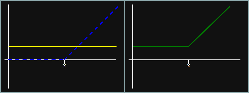
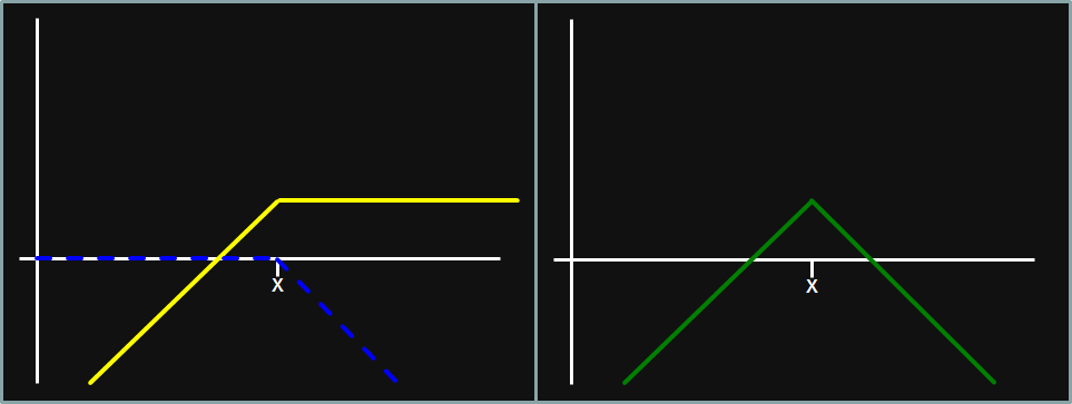
As an example, let’s return to investor S whose home currency is SEK and who has an investment denominated in NZD. The spot exchange rate is SEK/NZD 6.3744, and Investor S wants to hedge the SEK/NZD exchange rate for 6 months. As she is concerned that the SEK/NZD exchange rate will decrease (i.e., NZD will depreciate vis-à-vis SEK), she may buy 6-month put options on SEK/NZD with a strike price slightly below the current spot price (a protective put); say, SEK/NZD 6.0. Should the exchange rate fall below that strike price, the options will be in the money and investor S will exercise the options, limiting her loss to SEK/NZD 0.3744 (= SEK/NZD 6.3744 − SEK/NZD 6.0) on the contract amount of NZD, plus whatever premium she had to pay for the options. And if the exchange rate increases, she will benefit from that increase (less the premium she paid for the options).
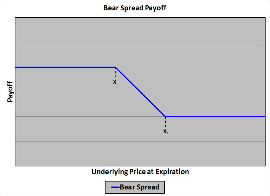
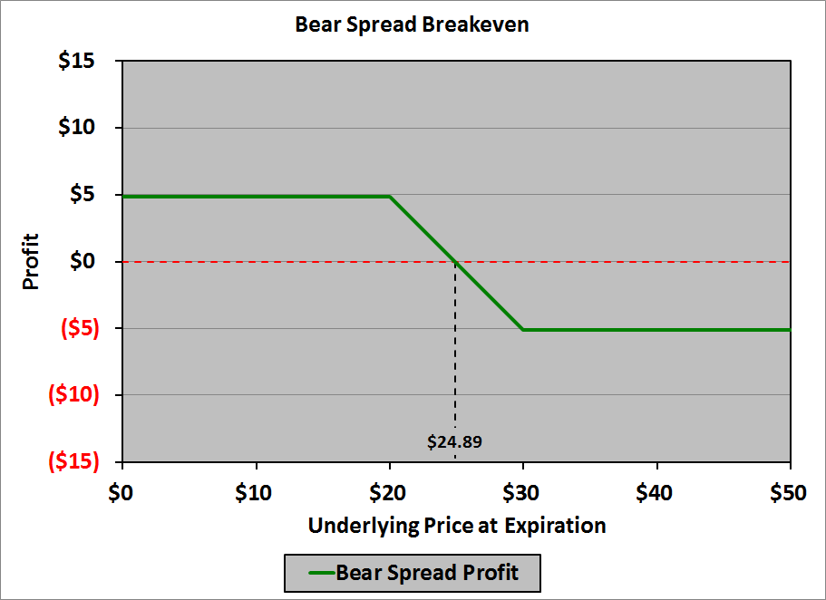
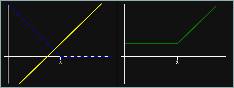
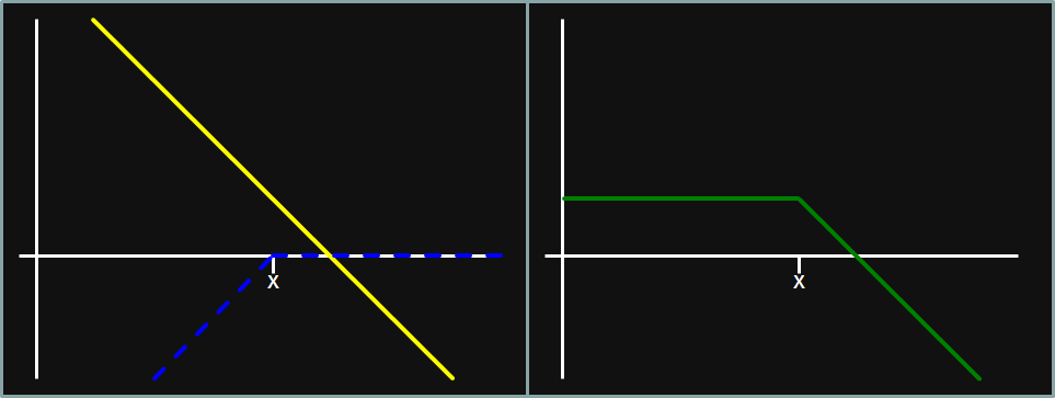
Alternatively, she could sell call options on SEK/NZD with a strike price above the spot price. The premium she receives for selling the options would offset at least some of the loss should the exchange rate decrease. However, should the exchange rate increase above the strike price on those call options, the option holder would exercise the options and she would lose any additional upside.
The advantage purchasing put options is that they set an absolute limit on the amount of loss, while providing the owner unlimited upside. The disadvantage is that they cost money, which will reduce the value of the investment irrespective of the value of the exchange rate at expiry.
The advantage of selling call options is that the premium received will offset some or all of the potential loss should the exchange rate decrease. The disadvantages are that they don’t provide an absolute limit to the amount of loss, and that they limit the potential gain should the exchange rate increase.
Exotic Options
There are many ways in which options can be “exotic”. One way is in the times at which the option can be exercised, which was mentioned above (Bermuda options and Canary options). Another way is in the manner in which the option comes into existence, or ceases to exist. Knock-in and knock-out options are considered exotic for that reason. A third way is in the manner in which the payoff on the option is determined. Digital options are considered exotic for that reason. I’ll discuss knock-in, knock-out, and digital options briefly. You’re not expected to do any calculations with these types of options; you’re expected only to know that they exist, how they differ (in general) from vanilla options, and generally why they might be used.
Knock-In Options
A knock-in option does not exist at the time it is written. (It’s probably more accurate to say that it exists, but is not active.) It comes into existence (is activated, or created) if and when the price of the underlying reaches a specified level (known as a barrier price; knock-in and knock-out options are examples of barrier options) before the option expires. For example, suppose that we have a spot price of SEK/NZD 6.3744. A knock-in call option may have a strike price of SEK/NZD 6.50 and a barrier price of SEK/NZD 6.00. At inception, the option is not active. It becomes active if and only if the spot price drops to SEK/NZD 6.00 or lower before expiry. If the spot price never drops that low, the option expires worthless. If the spot price does drop that low, then the option is created, and thereafter it behaves like a vanilla call option with the given strike price. Once created, if the spot price at expiry is above the strike price, then the option owner will exercise the option, and the profit will be the difference between the spot price and the strike price (multiplied by the base currency amount in the contract). Such an option would be known as a down-and-in option, because it is knocked in (comes into existence) when the underlying price goes down enough.
A knock-in put option may have a strike price of, say, SEK/NZD 6.00 and a barrier price of SEK/NZD 6.50. That option would be created if the spot price is ever SEK/NZD 6.50 or higher; if so, thereafter it acts like a vanilla put option with a strike price of SEK/NZD 6.00. Such an option would be known as an up-and-in option: it is knocked in when the underlying price goes up enough.
A knock-in option will be less expensive than an otherwise equivalent vanilla option because of the possibility that it may never be created. Apart from that, determining the price of a knock-in option is well beyond the scope of the Level III CFA curriculum.
Knock-Out Options
A knock-out option exists (i.e., is active), but will cease to exist if and when the price of the underlying reaches the barrier price before the option expires. For example, suppose that we have a spot price of SEK/NZD 6.3744. A knock-out call option may have a strike price of SEK/NZD 6.50 and a barrier price of SEK/NZD 6.00. At inception, the option exists. It ceases to exist if and only if the spot price drops to SEK/NZD 6.00 or lower before expiry. If the spot price never drops that low, the option behaves like a vanilla call option with the given strike price: if the spot price at expiry is above the strike price, then the option owner will exercise the option, and the profit will be the difference between the spot price and the strike price (multiplied by the base currency amount in the contract). Such an option would be known as a down-and-out option, because it is knocked out (ceases to existence) when the underlying price goes down enough.
A knock-out put option may have a strike price of, say, SEK/NZD 6.00 and a barrier price of SEK/NZD 6.50. That option would cease to exist if the spot price is ever SEK/NZD 6.50 or higher; if that never happens, then at expiry it acts like a vanilla put option with a strike price of SEK/NZD 6.00. Such an option would be known as an up-and-out option: it is knocked out when the underlying price goes up enough.
A knock-out option will be less expensive than an otherwise equivalent vanilla option because of the possibility that it may cease to exist before expiry. Apart from that, determining the price of a knock-out option is well beyond the scope of the Level III CFA curriculum.
Digital Options
A digital option is an all-or-nothing option: the payoff is zero if a specified event does not occur, and a fixed (nonzero) amount if that event occurs. For example, suppose that at 1:00 PM we have a spot price of SEK/NZD 6.3744. A digital call call option may have a strike price of SEK/NZD 6.38 with an expiry of 3:00 PM. If the spot SEK/NZD price at 3:00 PM is below 6.38, the payoff is zero, but if the spot SEK/NZD price at 3:00 PM is 6.38 or higher, then the option pays off a fixed amount (say, SEK 1 million). In many respects it’s like buying a lottery ticket.
Determining the price of a digital option is well beyond the scope of the Level III CFA curriculum.
Currency Swaps
At Levels I and II you learned that in a currency swap the notional amounts of the currencies are exchanged at the inception of the swap, then exchanged back at the maturity of the swap. You were taught that because you were a shorn lamb whose delicate nature had to be protected. The wind had to be tempered.
At Level III, you’re old enough and sophisticated enough to learn the truth: not all currency swaps involve the exchange of notional values at inception and maturity. I’ll give you a minute to recover from that revelation.
In some situations, it makes sense to exchange notionals. For example, suppose that investor C’s home currency is CHF, that they need to borrow THB 3 billion (three billion Thai baht) for a project, and that it’s cheaper for them to borrow CHF than THB. In that case, investor C might borrow CHF 81 billion (with the current spot rate at THB/CHF 37.1197) and enter into a CHF/THB currency swap, in which the notional values are exchanged at inception (investor C has CHF 81 million that they don’t want, so they exchange it for THB 3.01 billion that they do want), and again (in the opposite direction) at maturity.
In other situations, it does not. Suppose that investor C, above, needs to make quarterly rental payments on a warehouse in Angola in AOA (Angolan kwanza) for the next year. In that case they might enter into a CHF/AOA currency swap with quarterly settlement. There is no reason to exchange a notional amount at the inception or at the maturity.
There are, broadly, three types of currency swaps:
- Fixed-for-fixed: each party pays a fixed rate on a given notional amount in one currency, and receives a fixed rate on a given notional amount in another currency
- Fixed-for-floating: one party pays a fixed rate on a given notional amount in one currency, and the other party pays a floating rate on a given notional amount in another currency
- Floating-for-floating: each party pays a floating rate on a given notional amount in one currency, and receives a floating rate on a given notional amount in another currency
According to what you learned in Level II, the floating rates would be determined by each currency’s short-term rate (e.g., for a quarterly pay swap, they would be the 3-month LIBOR rates for each currency), and the fixed rates would be determined by each currency’s overall yield curve. (Determining the fixed rates is a Level II problem; you won’t have to do that here. Yippee!) A subtlety added at Level III is that there may be market forces at play other than the individual yield curves (e.g., more demand for one currency than another), so one of the payments may be adjusted up or down by a fixed amount, called the basis (or basis spread). (In fact, at Level III, we don’t call these merely currency swaps; they’re cross-currency basis swaps. Oooohhh! And a cross-currency basis swap always involves the exchange of notionals.) According to the curriculum, when USD is involved in a cross-currency basis swap, the basis is added to (or, if it’s negative, subtracted from) the other currency’s rate. What you’re to do for a GBP/CAD cross-currency basis swap with a basis of 21 bps, they don’t say. Presumably on the exam they’ll be explicit about which currency’s rate is adjusted by the basis.
For example, suppose that you enter into a 3-year, annual pay, fixed-for-fixed, cross-currency basis swap with a notional of GBP 50 million / CAD 77.9 million. At inception, you receive GBP 50 million in exchange for CAD 77.9 million. The GBP 12-month fixed rate is 2.4%, the CAD 12-month fixed rate is 1.8%, and the basis (which adjusts the CAD rate) is −45 bps. On each settlement date, you will pay 2.4% of GBP 50 million, or GBP 1,200,000, and you will receive 1.35% (= 1.80% − 0.45%) of CAD 77.9 million, or CAD 1,051,650.
Note that in the curriculum, they are not specific about how the basis is quoted for settlements that aren’t annual. They give one example in which they give the semiannual rate (that is, not annualized), and the semiannual basis (also not annualized), but they don’t say specifically what to do if the rate is quoted as an annual rate; i.e., is the basis also assumed to be an annual quote (so that you would have to divide it by 2 to get the basis for each payment). I trust that if this should appear on an exam, they’ll make it clear whether the basis is quoted for a 12-month period, or a 6-month period, or whatever.