A time-honored method to determine the value of an investment is to discount to the present all of the investment’s (expected) future cash flows, and tot up those present values.  It’s a method we use commonly when valuing bonds, and when valuing projects in which a company is considering investing (e.g., whether or not to purchase a machine that makes tennis balls): calculating the net present value (NPV), or, in a similar vein, its internal rate of return (IRR).  I describe these ideas in detail in this article.

Extending that idea to an investment in a company’s stock, when a company pays dividends regularly – and is expected to continue to pay dividends ad infinitum – a reasonable way to determine the value of the company’s stock is to use a dividend discount model (DDM): discount each of the expected dividends to the present (at your required rate of return) and tot up those present values; the resulting sum is the value of the stock (at least, its value to you).

Example

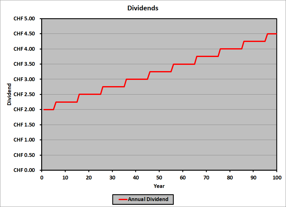
Euler Pharmaceuticals pays an annual dividend of CHF 2.00 per share.  Historically, they have raised their annual dividend by CHF 0.25 per share every 10 years; they have been paying the current dividend for the last 5 years.  Their expected dividends are:

Graphically:

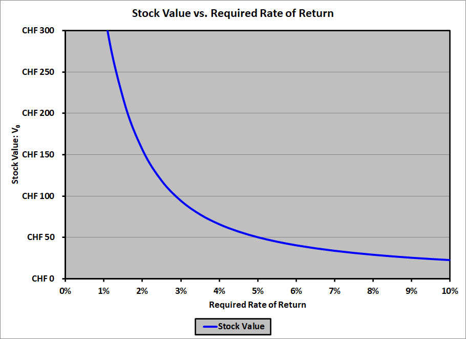
The value of the stock depends on the discount rate (required rate of return) used to determine the present value of the dividends.  The value versus the required rate of return is:

Graphically:

The problem with this (sort of) real-world example is that analyzing a dividend that increases every once in a while and otherwise remains constant is . . . um . . . difficult (unless you’re doing it in Excel, as I am).

Therefore, the curriculum makes some simplifying assumptions to make it easier to determine the value of a stock based on its expected dividends.  We acknowledge that these assumptions are unreasonable in the real world, but they make the models easy to understand.  Once you understand these simplified models thoroughly, it’s much easier to graduate to more complex (i.e., realistic) models and understand them.  So . . . tally ho!

(Short) Holding Period Models

We start with the most unrealistic model possible: you plan to buy a stock today, hold it for one year (receiving one dividend at the end of the year), then sell it.  You know your required rate of return, you know the dividend you’ll receive in one year, and you know the price at which you’ll be able to sell the stock in one year.  (That’s the unreasonable part: how can you possibly know the price at which you’ll sell the stock in one year without knowing its price today?)  You need to compute the price of the stock today.  Let’s look again at Euler Pharmaceuticals:

• Next year’s expected dividend: CHF 2.00
• Expected price in one year: CHF 31.52
• Required rate of return: 7.50%

The price you’d be willing to pay today is:

\begin{align}V_0\ &=\ \dfrac{D_1}{1 + r} + \dfrac{P_1}{1 + r}\\
\\
&=\ \dfrac{CHF\ 2.00}{1.075} + \dfrac{CHF\ 31.52}{1.075}\\
\\
&=\ CHF\ 1.86 + CHF\ 29.32\\
\\
&= CHF\ 31.18
\end{align}

Suppose, instead, that you plan to hold the stock for two years:

• Expected dividend in one year: CHF 2.00
• Expected dividend in two years: CHF 2.00
• Expected price in two years: CHF 31.88
• Required rate of return: 7.50%

The price you’d be willing to pay today is:

\begin{align}V_0\ &=\ \dfrac{D_1}{1 + r} + \dfrac{D_2}{\left(1 + r\right)^2} + \dfrac{P_2}{\left(1 + r\right)^2}\\
\\
&=\ \dfrac{CHF\ 2.00}{1.075} + \dfrac{CHF\ 2.00}{1.075^2} + \dfrac{CHF\ 31.88}{1.075^2}\\
\\
&=\ CHF\ 1.86 + CHF\ 1.73 + CHF\ 27.59\\
\\
&= CHF\ 31.18
\end{align}

Note that on your calculator, you can solve these with the TVM buttons.  For example, the second one can be solved this way: (with your calculator in END mode):

n = 2
i = 7.5%
PMT = 2.00
FV = 31.88
Solve for PV = −31.18

Single-Stage (Gordon Growth) Model

When the holding period is long-term (essentially, infinite, or perpetual), a common simplifying assumption is that the dividend grows at a constant rate.  The model incorporating this assumption is known as the Gordon Growth model, and the formula for the value of the stock is simplicity itself:

\begin{align}V_0\ &=\ \dfrac{D_1}{1 + r} + \dfrac{D_2}{\left(1 + r\right)^2} + \dfrac{D_3}{\left(1 + r\right)^3} + \cdots\\
\\
&= \sum_{i=1}^\infty \dfrac{D_i}{\left(1 + r\right)^i}\\
\\
&=\ \dfrac{D_0\left(1 + g\right)}{1 + r} + \dfrac{D_0\left(1 + g\right)^2}{\left(1 + r\right)^2} + \dfrac{D_0\left(1 + g\right)^3}{\left(1 + r\right)^3} + \cdots\\
\\
&= \sum_{i=1}^\infty \dfrac{D_0\left(1 + g\right)^i}{\left(1 + r\right)^i}\\
\\
V_0 &=\ \dfrac{D_0\left(1 + g\right)}{r\ -\ g} =\ \dfrac{D_1}{r\ -\ g}
\end{align}

where:

• \(r\): required rate of return
• \(g\): dividend growth rate

Note that this model makes sense only if \(r > g\).  Otherwise, the sum is infinite.

Let’s take a careful look at this formula, to see whether or not it makes sense.  We’ll compare the stocks of two companies, not particularly cleverly known as Company A and Company B.

D₁

Suppose first that the stocks of Companies A and B are considered equally risky (so that they command the same required rate of return), and that their dividends will grow at the same rate unto perpetuity.  Company A just paid a dividend of GBP 1.00 while Company B just paid a dividend of GBP 1.25.  I hope that it’s clear that you would be willing to pay more for Company B’s stock than for Company A’s stock, and that’s exactly what we get from the Gordon Growth formula: when D₀ (and, consequently, D₁) is higher, all else equal, V₀ is higher (because the numerator is bigger and the denominator is unchanged), and conversely.

r

Suppose now that Companies A and B just paid the same dividend, and that their dividends will grow at the same rate unto perpetuity, but that Company B’s stock is considered riskier than Company A’s stock.  I trust that it’s clear that your required rate of return for Company B’s stock will be higher than your required rate of return for Company A’s stock, and that, therefore, you would be willing to pay less for Company B’s stock than for Company A’s stock.  We see that that’s exactly what we get from the Gordon Growth formula: when r is higher, all else equal, V₀ is lower (because the numerator is unchanged while the denominator is bigger), and conversely.

g

Suppose now that Companies A and B just paid the same dividend, and are considered equally risky, but that Company B’s dividend is expected to increase at a faster rate than Company A’s dividend.  I assume that it’s clear that you would be willing to pay more for Company B’s stock than for Company A’s stock.  We see that that’s exactly what we get from the Gordon Growth formula: when g is higher, all else equal, V₀ is higher (because the numerator is unchanged while the denominator is smaller), and conversely.

In all cases, the Gordon Growth model passes muster: it behaves exactly as we should expect it to behave, and the analyses are simple and straightforward.  That’s the point of making these simplifying assumptions: it’s easy to understand how the model works, and it works the way it’s meant to work.  Once we understand that, presumably we can move on to more complex (and reasonable) models and be able to understand how they work as well.

Example

Suppose that Ramanujan Technologies just paid an annual dividend of INR 200.00 per share.  Its dividends are expected to grow at 1.5% per year, and you determine that 8.4% is an appropriate rate of return for such an investment.  The amount per share you should be willing to pay for Ramanujan Technologies stock is:

\[V_0 = \dfrac{D_1}{r\ -\ g} = \dfrac{INR\ 200 \times 1.015}{0.084\ -\ 0.015} = INR\ 2,942.03\]

Delayed Gordon Growth Model

Suppose that instead of the first dividend coming one year from today, we expect the first dividend five years from today; i.e., the company does not pay a dividend yet, but we expect that it will start paying one in five years (and that the dividend will grow at a constant rate thereafter).  Before we analyze the value of the company’s stock, let’s take another look at the Gordon Growth model:

\[V_0 = \dfrac{D_1}{r\ -\ g}\]

There’s nothing special about the subscript “0” on the value, or the subscript “1” on the dividend; what’s important is that the dividend comes one year after the date for the value.  So, for example,

\[V_1 = \dfrac{D_2}{r\ -\ g}\]

\[V_2 = \dfrac{D_3}{r\ -\ g}\]

and, in general,

\[V_t = \dfrac{D_{t+1}}{r\ -\ g}\]

Therefore, we can use the Gordon Growth model to determine the value of the stock one year before the first dividend is paid.  If the date on the value isn’t today, then we simply discount that value back to today.

Example

Suppose that Abel Industrial is expected to start paying a dividend five years from today.  The first (annual) dividend is anticipated to be EUR 2.50 per share, increasing 1% per year thereafter.  If your required rate of is 8.2%, how much would you be willing to pay for a share of Abel stock?

\begin{align}V_4\ &=\ \dfrac{D_5}{r\ -\ g}\\
\\
&= \dfrac{EUR\ 2.50}{8.2\%\ -\ 1.0\%}\\
\\
V_4 &= EUR\ 34.72\\
\\
V_0 &= \dfrac{V_4}{\left(1 + r\right)^4}\\
\\
&= \dfrac{EUR\ 34.72}{1.082^4}\\
\\
&=\ EUR\ 25.33
\end{align}

Multi-Stage Models

In a two-stage growth model, a company’s dividends are assumed to grow a one rate (presumably a high rate) for a finite period of time, then to grow at another rate (presumably a lower rate) forever thereafter.  In a three-stage growth model, the dividends are assumed to grow at one (high) rate for a finite period of time, then at a second (middling) rate for another finite period of time, then at a third (low) rate forever thereafter.  I’ll leave it to your imagination what a four-stage, or a five-stage, or a six-stage, or a more-than-six-stage model might be.

The approach for determining the value of the company’s stock under all of these models is the same:

• Determine all of the dividend amounts for all of the finite periods
• Discount those amounts to the present
• Use the Delayed Gordon Growth model for the final (infinite) period
• Tot up all of the present values
• Voilà!

Two-Stage Example

Jacobi Materials just paid an annual dividend of EUR 1.75 per share.  They expect the dividend to grow 10% per year for the next five years, then to grow at 2% per year forever thereafter.  If you require a return of 7.7% to invest in Jacobi, how much would you be willing to pay for a share of its stock today?

The dividends for the first six years will be:

The value is computed as:

\begin{align}V_0\ &=\ \left[\sum_{i=1}^5 \dfrac{D_i}{\left(1 + r\right)^i}\right] + \dfrac{D_6}{\left(r\ -\ g_{low}\right)\left(1 + r\right)^5}\\
\\
&= \dfrac{EUR\ 1.925}{1.077} + \dfrac{EUR\ 2.1175}{1.077^2} + \cdots + \dfrac{EUR\ 2.8184}{1.077^5} + \dfrac{EUR\ 2.8748}{\left(7.7\%\ -\ 2\%\right)1.077^5}\\
\\
&=\ EUR\ 44.13
\end{align}

(Note that you could add the discounted values of the first four dividends, then use the Delayed Gordon Growth formula on the fifth dividend and arrive at the same total.  Just an interesting fact.)

Three-Stage Example

Dirichlet Products just paid an annual dividend of EUR 2.25 per share.  They expect the dividend to grow 10% per year for the next three years, then to grow at 5% for two more years, then to grow at 2% per year forever thereafter.  If you require a return of 7.3% to invest in Dirichlet , how much would you be willing to pay for a share of its stock today?

The dividends for the first few years will be:

The value is computed as:

\begin{align}V_0\ &=\ \left[\sum_{i=1}^5 \dfrac{D_i}{\left(1 + r\right)^i}\right] + \dfrac{D_6}{\left(r\ -\ g_{low}\right)\left(1 + r\right)^5}\\
\\
&= \dfrac{EUR\ 2.475}{1.073} + \dfrac{EUR\ 2.7225}{1.073^2} + \cdots + \dfrac{EUR\ 3.1516}{1.073^5} + \dfrac{EUR\ 3.2147}{\left(7.3\%\ -\ 2\%\right)1.073^5}\\
\\
&=\ EUR\ 54.11
\end{align}

(Note that, again, you could add the discounted values of the first four dividends, then use the Delayed Gordon Growth formula on the fifth dividend and arrive at the same total.)

Combining Dividend Discount Models and Multiplier Models

Occasionally, an analyst will combine a dividend discount model with a multiplier model: the terminal value is computed using a multiplier rather than using the Gordon Growth model.  It’s not a big deal.

Example

Suppose that Dedekind Cutlery just paid a dividend of EUR 1.25 per share, which was 50% of its earnings per share (EPS).  Its EPS is expected to grow at 4% per year for the next five years (with its payout ratio remaining constant), whereupon its trailing P/E ratio is expected to be 15.4.  If you require a return of 8.1% to invest in Dedekind, how much would you be willing to pay for a share of its stock today?

The earnings and dividends for the next five years are expected to be:

The share price five years from today is expected to be:

\[V_5 = EUR\ 3.0146 \times 15.4 = EUR\ 46.84\]

Today’s value is calculated as:

\begin{align}V_0\ &=\ \left[\sum_{i=1}^5 \dfrac{D_i}{\left(1 + r\right)^i}\right] + \dfrac{V_5}{\left(1 + r\right)^5}\\
\\
&= \dfrac{EUR\ 1.30}{1.081} + \dfrac{EUR\ 1.352}{1.081^2} + \cdots + \dfrac{EUR\ 1.5208}{1.081^5} + \dfrac{EUR\ 46.84}{1.081^5}\\
\\
&=\ EUR\ 37.31
\end{align}

When to Use a Dividend Discount Model

A valid question to ask is, “When should I use a dividend discount model to estimate the value of a stock?”

Obviously, a necessary condition for using a DDM is that the company pays a dividend; either it pays one now, or it is expected to start paying one in the foreseeable future, and that it will continue to pay dividends.

Assuming that that criterion is met, why use a DDM instead of, say, a free cash flow model?  The general answer is that dividends tend to be more stable than either free cash flow to equity (FCFE) or free cash flow to the firm (FCFF), so they’re more easily predicted (i.e., estimated).  This is certainly true for the way that most companies pay dividends: their dividend remains constant over a period of time, and they raise it only when they reasonably expect that they will be able to maintain the new (higher) dividend into the future.

However, if, instead of maintaining a constant dividend amount, a company chooses to pay a dividend amounting to a constant percentage of its net income, its FCFE, or its FCFF, then there’s no particular advantage to using a DDM over a FCFE model or a FCFF model.  And if they’re even less disciplined – their dividends being based on little more than whim and caprice (“Oh, what the heck?  Let’s pay a dividend!  Just for giggles!”) – then a DDM is even less likely to be an appropriate valuation model.