An equity index is nothing more nor less than a hypothetical stock portfolio. The index pretends to invest in a bunch of stocks, and tracks their performance over time. It’s the sort of thing that you may have done in a high school economics or history class. I did, at least.
I don’t intend to cover the uses of equity indices – benchmarking portfolio managers’ performances, measuring market sentiment, and so on – that’s easy stuff that you can cover on your own.
What I want to cover is the mechanics of constructing these indices, their inherent biases, and the issues in constructing portfolios to track these indices.
For our purposes, there are three broad types of equity indices:
- Price-weighted indices
- Value-weighted (or cap-weighted) indices
- Equal-weighted (or unweighted) indices
A fourth category of indices – fundamental-weighted indices – is starting to gain some popularity, but at the moment it lags far behind the big three; I won’t cover that category here.
Data
To compare the three index types, we’ll use the same data for each. Here they are:
Our indices each comprise three stocks: A, B, and C. Initially, there are 5,000,000 shares of stock A outstanding, 20,000,000 shares of stock B outstanding, and 10,000,000 shares of stock C outstanding; apart from the stock split in year 6, no shares were issued or repurchased. The prices of the constituent stocks are:
| Year |
Stock A |
Stock B |
Stock C |
| 0 |
$95.44 |
$22.37 |
$44.21 |
| 1 |
$93.23 |
$20.43 |
$45.08 |
| 2 |
$92.96 |
$20.68 |
$45.71 |
| 3 |
$103.25 |
$19.68 |
$45.57 |
| 4 |
$90.29 |
$18.21 |
$45.57 |
| 5 |
$98.22 |
$19.64 |
$45.99 |
| 6 |
$59.45* |
$21.59 |
$45.99 |
| 7 |
$56.57 |
$22.59 |
$45.99 |
| 8 |
$55.83 |
$22.79 |
$45.94 |
| 9 |
$58.96 |
$24.42 |
$46.12 |
| 10 |
$64.62 |
$24.90 |
$46.35 |
*In year 6, stock A split 2:1
All three indices will have a starting value of 100.
Price-Weighted Indices
In a price-weighted index, the hypothetical portfolio contains the same number of shares of each stock; you can think of it as owning a single share of each. The formula to determine the value of the index at any time t is:
\[Time-Weighted\ Index_t\ =\ \dfrac{\sum_{i=1}^nP_{i_t}}{D_t}\]
where:
- \(n\): number of stocks in the index
- \(P_{i_t}\): share price of stock i at time t
- \(D_t\): divisor at time t
The divisor \(D_t\) is adjusted for stock splits, reverse stock splits, stock dividends, and changes in the stocks in the index. I’ll show you how the divisor is calculated initially (i.e., when the index is first created), and how it is adjusted for the items mentioned. It’s not difficult.
Initial Divisor: D0
Most indices are given some nice, round number as a starting point: 100, 500, 1,000, that sort of thing. Some simple arithmetic is all that’s necessary to determine the divisor that will generate the desired starting index value. Let’s use the example data with a starting index value of 100:
\begin{align}100\ &=\ \dfrac{\$95.44\ +\ \$22.37\ +\ \$44.21}{D_0}\\
\\
100D_0\ &=\ \$162.02\\
\\
D_0\ &=\ \dfrac{\$162.02}{100}\ =\ \$1.6202
\end{align}
This divisor is used until one of the items mentioned (i.e., a stock split, reverse stock split, stock dividend, or change in stock in the index) occurs. Using our example data,
\[Price-Weighted\ Index_0\ =\ \dfrac{\$95.44\ +\ \$22.37\ +\ \$44.21}{\$1.6202}\ =\ 100.00\]
\[Price-Weighted\ Index_1\ =\ \dfrac{\$93.23\ +\ \$20.43\ +\ \$45.08}{\$1.6202}\ =\ 97.98\]
\[Price-Weighted\ Index_2\ =\ \dfrac{\$92.96\ +\ \$20.68\ +\ \$45.71}{\$1.6202}\ =\ 98.35\]
\[Price-Weighted\ Index_3\ =\ \dfrac{\$103.25\ +\ \$19.68\ +\ \$45.57}{\$1.6202}\ =\ 104.00\]
\[Price-Weighted\ Index_4\ =\ \dfrac{\$90.29\ +\ \$18.21\ +\ \$45.57}{\$1.6202}\ =\ 95.09\]
\[Price-Weighted\ Index_5\ =\ \dfrac{\$98.22\ +\ \$19.64\ +\ \$45.99}{\$1.6202}\ =\ 101.13\]
Recalculating the Divisor
When one of the items mentioned (i.e., a stock split, reverse stock split, stock dividend, or change in stock in the index) occurs, we have to recalculate the divisor. The idea is that the value of the index should not change simply because one of these events occurs: there is no economic event happening; it’s only an accounting phenomenon.
Let’s look at our example data: in year 6, stock A undergoes a 2:1 split. Thus, the share price of stock A will be cut in half, but no economic event has occurred. We need to recalculate the divisor (based on year 5 data) so that the value of the index remains unchanged (at 101.13):
\begin{align}101.13\ &=\ \dfrac{\$95.44/2\ +\ \$22.37\ +\ \$44.21}{D_5}\\
\\
101.13D_5\ &=\ \$114.74\\
\\
D_5\ &=\ \dfrac{\$114.74}{101.13}\ =\ \$1.1346
\end{align}
Once again, this divisor is used until one of the items mentioned occurs:
\[Price-Weighted\ Index_6\ =\ \dfrac{\$54.45\ +\ \$21.59\ +\ \$45.99}{\$1.1346}\ =\ 111.96\]
\[Price-Weighted\ Index_7\ =\ \dfrac{\$56.47\ +\ \$22.59\ +\ \$45.99}{\$1.1346}\ =\ 110.30\]
\[Price-Weighted\ Index_8\ =\ \dfrac{\$55.83\ +\ \$22.79\ +\ \$45.94}{\$1.1346}\ =\ 109.78\]
\[Price-Weighted\ Index_9\ =\ \dfrac{\$58.96\ +\ \$24.42\ +\ \$46.12}{\$1.1346}\ =\ 114.14\]
\[Price-Weighted\ Index_{10}\ =\ \dfrac{\$64.52\ +\ \$24.90\ +\ \$46.35}{\$1.1346}\ =\ 119.75\]
Notice, in particular, that we recalculate the divisor at the beginning of the period in which the change occurs. Here, the change (the stock split) occurs in period 6, so we recalculate the divisor as if the split occurred at the beginning of period, which is the end of period 5, leaving the time 5 index value unchanged.
Here’s how the index value looks over time:
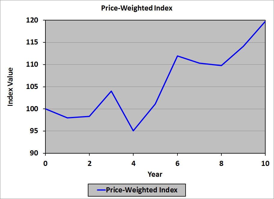
Bias
Price-weighted indices are biased toward the stocks with the highest share price: a 1% change in a $100/share stock will have a much greater effect on the index than a 1% change in a $10/share stock.
Examples
The Dow Jones Industrial Average (DJIA) and the Nikkei index are price-weighted equity indices.
Issues in Constructing Tracking Portfolios
Because (the divisor for) a price-weighted index needs to be recalculated whenever a constituent stock undergoes a stock split, undergoes a reverse stock split, or issues a stock dividend, or is replaced by another company’s stock, a tracking portfolio will have to make adjustments for all of these events as well. In particular, if a constituent stock undergoes a stock split or issues a stock dividend, a tracking portfolio will have more shares in that stock than in the other stocks and will therefore have to sell shares. If a constituent stock undergoes a reverse stock split, a tracking portfolio will have fewer shares in that stock than in the other stocks and will therefore have to buy shares. If one stock in the index is replaced with another stock, a tracking portfolio will have to sell all of its shares in the former and purchase the same number of shares in the latter.
Value-Weighted Indices
In a value-weighted index, the hypothetical portfolio contains all available shares of each stock. There are two subcategories of value-weighted indices:
- Unadjusted for free-float
- Adjusted for free-float
Unadjusted for Free-Float
When a value-weighted index is not adjusted for free-float, the number of shares of each stock included in the index is the total number of shares issued and outstanding. The formula to determine the value of the index at any time t is:
\[Value-Weighted\ Index_t\ =\ \left(\dfrac{\sum_{i=1}^nP_{i_t}Q_{i_t}}{\sum_{i=1}^nP_{i_b}Q_{i_b}}\right)\left(Beginning\ Index\ Value\right)\]
where:
- \(n\): number of stocks in the index
- \(P_{i_t}\): share price of stock i at time t
- \(Q_{i_t}\): number of shares of stock i at time t
- \(P_{i_b}\): share price of stock i outstanding at time b (beginning: when the index started)
- \(Q_{i_b}\): number of shares of stock i outstanding at time b (beginning, when the index started)
The nice thing about value-weighted indices is that you don’t need to make any adjustments when there is a stock split, reverse stock split, or stock dividend: the total value of the outstanding stock doesn’t change when these events occur.
The divisor is the total market capitalization of all stocks in the index when the index originates. Using our example data:
\begin{align}Divisor\ &=\ \sum_{i=1}^nP_{i_b}Q_{i_b}\\
\\
&=\ \$95.44\left(5,000,000\right)\ +\ \$22.37\left(20,000,000\right)\\
\\
&+\ \$44.21\left(10,000,000\right)\\
\\
&=\ \$1,366,700,000
\end{align}
The total market capitalization at each time is:
\begin{align}Time\ 0:\ \$95.44\ ×\ 5,000,000\ &+\ \$22.37\ ×\ 20,000,000\\
&+\ \$44.21\ ×\ 10,000,000\ =\ \$1,366,700,000\\
\\
Time\ 1:\ \$93.23\ ×\ 5,000,000\ &+\ \$20.43\ ×\ 20,000,000\\
&+\ \$45.08\ ×\ 10,000,000\ =\ \$1,325,550,000\\
\\
Time\ 2:\ \$92.96\ ×\ 5,000,000\ &+\ \$20.68\ ×\ 20,000,000\\
&+\ \$45.71\ ×\ 10,000,000\ =\ \$1,335,500,000\\
\\
Time\ 3:\ \$103.25\ ×\ 5,000,000\ &+\ \$19.68\ ×\ 20,000,000\\
&+\ \$45.57\ ×\ 10,000,000\ =\ \$1,365,550,000\\
\\
Time\ 4:\ \$90.29\ ×\ 5,000,000\ &+\ \$18.21\ ×\ 20,000,000\\
&+\ \$45.57\ ×\ 10,000,000\ =\ \$1,271,350,000\\
\\
Time\ 5:\ \$98.22\ ×\ 5,000,000\ &+\ \$19.64\ ×\ 20,000,000\\
&+\ \$45.99\ ×\ 10,000,000\ =\ \$1,343,800,000\\
\\
Time\ 6:\ \$59.45\ ×\ 10,000,000\ &+\ \$21.59\ ×\ 20,000,000\\
&+\ \$45.99\ ×\ 10,000,000\ =\ \$1,486,200,000\\
\\
Time\ 7:\ \$56.57\ ×\ 10,000,000\ &+\ \$22.59\ ×\ 20,000,000\\
&+\ \$45.99\ ×\ 10,000,000\ =\ \$1,477,400,000\\
\\
Time\ 8:\ \$55.83\ ×\ 10,000,000\ &+\ \$22.79\ ×\ 20,000,000\\
&+\ \$45.94\ ×\ 10,000,000\ =\ \$1,473,500,000\\
\\
Time\ 9:\ \$58.96\ ×\ 10,000,000\ &+\ \$24.42\ ×\ 20,000,000\\
&+\ \$46.12\ ×\ 10,000,000\ =\ \$1,539,200,000\\
\\
Time\ 10:\ \$64.62\ ×\ 10,000,000\ &+\ \$24.90\ ×\ 20,000,000\\
&+\ \$46.35\ ×\ 10,000,000\ =\ \$1,607,700,000\\
\end{align}
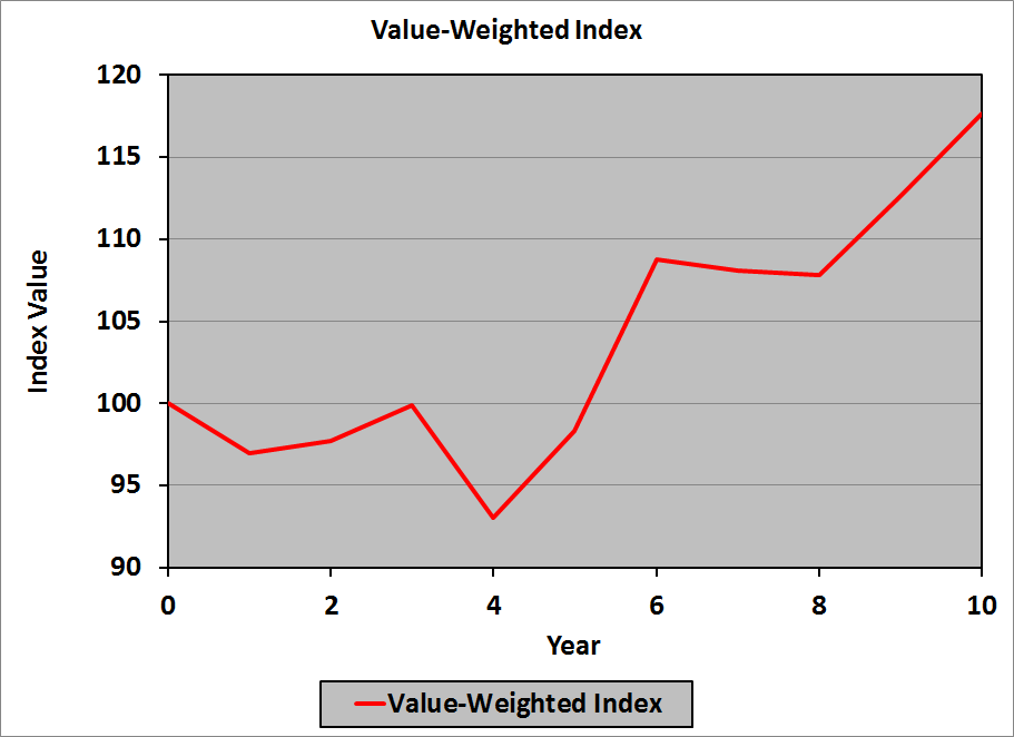
The corresponding index values are:
\begin{align}Time\ 0:\ \dfrac{\$1,366,700,000}{\$1,366,700,000}\ &=\ 100.00\\
\\
Time\ 1:\ \dfrac{\$1,325,550,000}{\$1,366,700,000}\ &=\ 96.99\\
\\
Time\ 2:\ \dfrac{\$1,335,500,000}{\$1,366,700,000}\ &=\ 97.72\\
\\
Time\ 3:\ \dfrac{\$1,365,550,000}{\$1,366,700,000}\ &=\ 99.92\\
\\
Time\ 4:\ \dfrac{\$1,271,350,000}{\$1,366,700,000}\ &=\ 93.02\\
\\
Time\ 5:\ \dfrac{\$1,343,800,000}{\$1,366,700,000}\ &=\ 98.32\\
\\
Time\ 6:\ \dfrac{\$1,486,200,000}{\$1,366,700,000}\ &=\ 108.74\\
\\
Time\ 7:\ \dfrac{\$1,477,400,000}{\$1,366,700,000}\ &=\ 108.10\\
\\
Time\ 8:\ \dfrac{\$1,473,500,000}{\$1,366,700,000}\ &=\ 107.81\\
\\
Time\ 9:\ \dfrac{\$1,539,200,000}{\$1,366,700,000}\ &=\ 112.62\\
\\
Time\ 10:\ \dfrac{\$1,607,700,000}{\$1,366,700,000}\ &=\ 117.63
\end{align}
Here’s how the index value looks over time:
Adjusted for Free-Float
Many companies have common shares which, although issued and outstanding, are not available to the general public for purchase. One example of such shares would be those owned by the founders of the company, who have no intention of selling their shares. Another example is corporate cross-holdings: two companies that are closely allied will purchase shares of each other, to demonstrate their solidarity; once again, these companies have no intention of selling their shares in each other.
The free-float adjustment recognizes these shares as being unavailable to the investing public: each company in a free-float adjusted, value-weighted index has an associated free-float factor (FFF): a number between zero and one that gives the percentage of outstanding shares that are available for the investing public to purchase. The formula to determine the value of the free-float-adjusted index at any time t is:
\[Value-Weighted\ Index_t\ =\ \left(\dfrac{\sum_{i=1}^nP_{i_t}Q_{i_t}FFF_{i_t}}{\sum_{i=1}^nP_{i_b}Q_{i_b}FFF_{i_b}}\right)\left(Beginning\ Index\ Value\right)\]
where:
- \(FFF_{i_t}\): free-float factor for stock i at time t
- \(FFF_{i_b}\): free-float factor for stock i at time b
Bias
Value-weighted indices are biased toward the stocks with the highest market capitalization: a 1% change in a $100 million market cap stock will have a much greater effect on the index than a 1% change in a $10 million market cap stock.
Examples
The S&P 500, the NASDAQ, and the Wilshire 5000 indices are value-weighted equity indices.
Issues in Constructing Tracking Portfolios
Because a value-weighted index is not affected by stock splits, reverse stock splits, and stock dividends, a tracking portfolio will not have to make any adjustments for these events. However, if one stock in the index is replaced with another stock, a tracking portfolio will have to sell all of its shares in the former and purchase an appropriate number of shares in the latter.
Equal-Weighted (or Unweighted) Indices
In an equal-weighted index, the hypothetical portfolio contains the same dollar (euro, yen, baht, pound, whatever) value of each stock; you can think of it as owning $1.00 worth of each (or €1.00 worth of each, or £1.00 worth of each, or . . . well . . . you get the idea). The formula to determine the value of the index at any time t is:
\[Equal-Weighted\ Index_t\ =\ Index_{t-1}\left[1\ +\ \dfrac{\sum_{i=1}^n\left(\dfrac{P_{i_t}}{P_{i_{t-1}}}\ -\ 1\right)}{n}\right]\]
To understand the formula (which isn’t as difficult as it looks), note that \(\dfrac{P_{i_t}}{P_{i_{t-1}}}\ -\ 1\) is simply the return on stock i from time t − 1 to time t. We sum those and divide by n to get the average return on all stocks from time t − 1 to time t. We add that average return to 1 and multiply it by the previous index value: all we’ve done is increase the index value at time t − 1 by the average return.
Voilà!
The returns for each stock for year 1, and the average return for year 1, are computed as:
Stock A’s return:
\[\dfrac{\$93.23}{\$95.44}\ -\ 1\ =\ -2.32\%\]
Stock B’s return:
\[\dfrac{\$20.43}{\$22.37}\ -\ 1\ =\ -8.67\%\]
Stock C’s return:
\[\dfrac{\$45.08}{\$44.21}\ -\ 1\ =\ 1.97\%\]
Average return:
\[\dfrac{-2.32\%\ +\ -8.67\%\ +\ 1.97\%}{3}\ =\ -3.01\%\]
The returns for the constituent stocks for all of the years, and the corresponding average returns, are calculated similarly:
| Year |
Stock A |
Stock B |
Stock C |
Return A |
Return B |
Return C |
Avg. Return |
| 0 |
$95.44 |
$22.37 |
$44.21 |
— |
— |
— |
— |
| 1 |
$93.23 |
$20.43 |
$45.08 |
−2.32% |
−8.67% |
1.97% |
−3.01% |
| 2 |
$92.96 |
$20.68 |
$45.71 |
−0.29% |
1.22% |
1.40% |
0.78% |
| 3 |
$103.25 |
$19.68 |
$45.57 |
11.07% |
−4.84% |
−0.31% |
1.98% |
| 4 |
$90.29 |
$18.21 |
$45.57 |
−12.55% |
−7.47% |
0.00% |
−6.67% |
| 5 |
$98.22 |
$19.64 |
$45.99 |
8.78% |
7.85% |
0.92% |
5.85% |
| 6 |
$59.45 |
$21.59 |
$45.99 |
21.05%* |
9.93% |
0.00% |
10.33% |
| 7 |
$56.57 |
$22.59 |
$45.99 |
−4.84% |
4.63% |
0.00% |
−0.07% |
| 8 |
$55.83 |
$22.79 |
$45.94 |
−1.31% |
0.89% |
−0.11% |
−0.18% |
| 9 |
$58.96 |
$24.42 |
$46.12 |
5.61% |
7.15% |
0.39% |
4.38% |
| 10 |
$64.62 |
$24.90 |
$46.35 |
9.60% |
1.97% |
0.50% |
4.02% |
*The year 6 return on stock A is calculated using $59.45 as the new price and $49.11 (= $98.22 / 2) as the old price, given the 2:1 split.
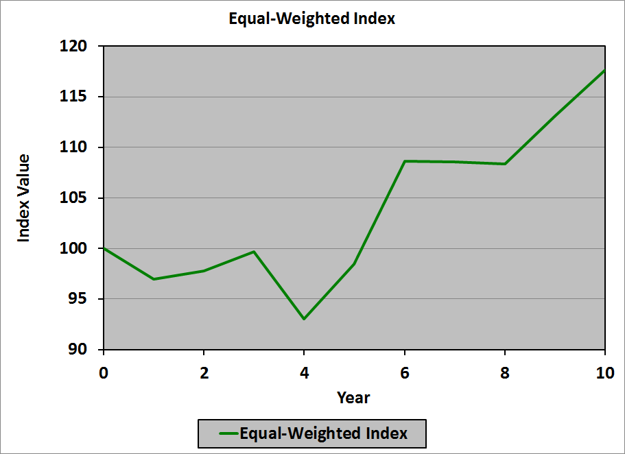
The corresponding index values are:
\begin{align}EWI_0\ &=\ 100.00\\
\\
EWI_1\ =\ 100.00\left(1\ +\ -3.01\%\right)\ &=\ 96.99\\
\\
EWI_2\ =\ 96.99\left(1\ +\ 0.78\%\right)\ &=\ 97.75\\
\\
EWI_3\ =\ 97.75\left(1\ +\ 1.98\%\right)\ &=\ 99.68\\
\\
EWI_4\ =\ 99.68\left(1\ +\ -6.67\%\right)\ &=\ 93.03\\
\\
EWI_5\ =\ 93.03\left(1\ +\ 5.85\%\right)\ &=\ 98.47\\
\\
EWI_6\ =\ 98.47\left(1\ +\ 10.33\%\right)\ &=\ 108.64\\
\\
EWI_7\ =\ 108.64\left(1\ +\ -0.07\%\right)\ &=\ 108.56\\
\\
EWI_8\ =\ 108.56\left(1\ +\ -0.18\%\right)\ &=\ 108.37\\
\\
EWI_9\ =\ 108.37\left(1\ +\ 4.38\%\right)\ &=\ 113.12\\
\\
EWI_{10}\ =\ 113.12\left(1\ +\ 4.02\%\right)\ &=\ 117.67\\
\end{align}
Here’s how the index value looks over time:
Bias
Equal-weighted indices are biased toward the stocks that have the highest volatility of returns. Because small-cap stocks tend to have higher volatility of returns than large-cap stocks, equal-weighted indices tend to be biased toward the returns of small-cap stocks.
Examples
The Value Line Index and the Financial Times Ordinary Share Index are equal-weighted equity indices.
Issues in Constructing Tracking Portfolios
Because an equal-weighted index assumes the same value held in each stock, it is impractical to create a true tracking portfolio for such an index. Every day the value of each security will change, so every day a tracking portfolio would have to rebalance back to equal weights, likely buying or selling fractions of shares of every stock it holds. Apart from the impossibility of selling fractions of shares, transactions costs would be prohibitive.
As a practical approximation, therefore, portfolios that attempt to track equal-weighted indices rebalance much less frequently: usually quarterly. Therefore, the weights on the securities in the portfolio will not be equal, so there will be differences in the performance of the portfolio and that of the index.
Oh, well.
Comparison of Index Values
Here’s how the index values look over time:
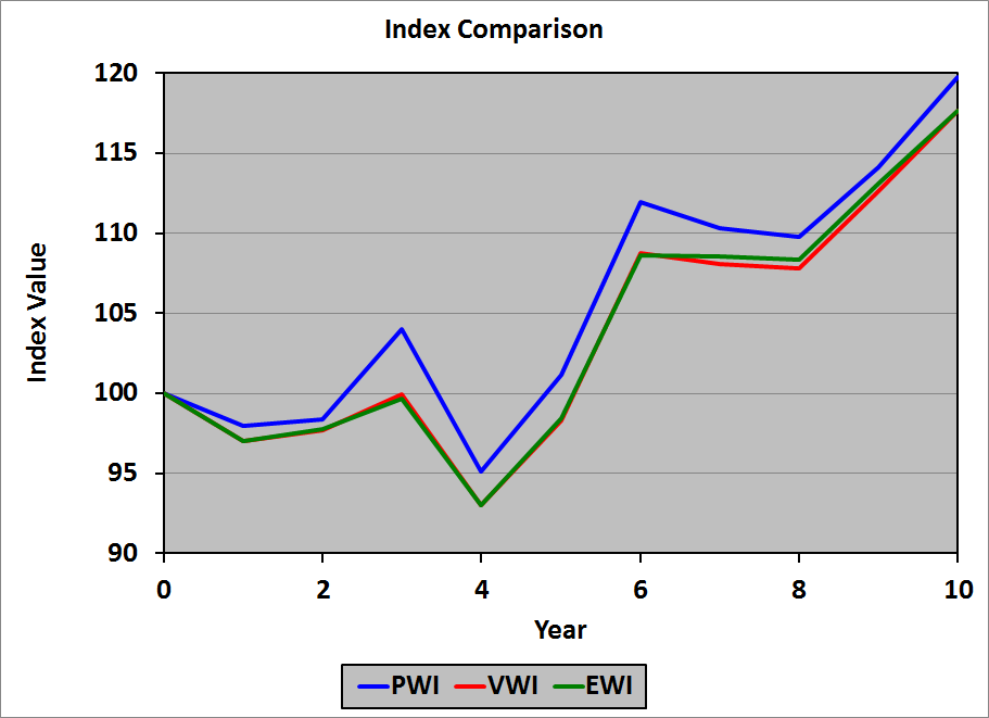
Note that the strong influence of stock A (with the highest share price, even after the split) in the price-weighted index is quite evident in the comparison.